November 2025 – PROCESS announces the official opening of a new engineering regional office in Greenville, SC. This office is being opened to better serve Southeastern clients in markets such as chemicals, polymers, food and beverage, etc. The office will be managed by Mr. Matt Whitworth, P.E.
Process Engineer at Process Engineering Associates
May 12, 2025
One common decision made during the front-end engineering and design (FEED) of a project is selecting the appropriate means of heat transfer to and from the process. However, selecting a heat transfer fluid can feel difficult due to the many options available. This article outlines the benefits and drawbacks of the most common heat transfer fluids and quantitatively compares various heat transfer fluids for heating, cooling, and refrigeration service.
Introduction
Heat transfer fluids are used for a variety of services in the process industry such as:
Fluid heating and vaporization
Fluid cooling, condensing, and crystallization
Reboiling liquids for distillation
Combined Heating and Cooling of Batch Systems
And many other additional services
The variety of process conditions encountered in the process industry means that the optimal heat transfer fluids may be different for each situation. Proper selection of heat transfer fluids results in lower capital and operating costs, and process engineers should evaluate the choice of heat transfer fluid carefully. The sections below describe the benefits and drawbacks of the most common fluids to help provide a guide for selecting a good heat transfer fluid.
Steam
Steam is an inexpensive and widely available heat transfer fluid. Due to its high film coefficient, using steam often results in smaller heat exchanger sizes. Steam is also available at most process plants and, if additional boiler capacity is available, it can be a very economical option.
Steam is quite useful for heating fluids to temperatures as high as 450°F. However, as process temperature requirements increase past 450°F, the applicability of steam becomes problematic. The vapor pressure of steam increases exponentially, and very high pressure is required to meet process temperatures above 450oF. For example, saturated steam at 600°F has a vapor pressure of ~1,530 psig. A typical hot oil system operating at the same temperature will often operate below 150 psig. Thus, using steam for high temperature applications often requires more expensive equipment and piping compared to other available heat transfer fluid options.
Another item that should be considered with steam use is when steam is being used in a dual-use jacket or coil, which are commonly applied to batch reactors. Dual-use jackets use steam for heating and then switch to cooling water service for cooling. Swapping between steam and cooling water, for example, can lead to hammering in equipment jackets and coils due to the rapid condensation of steam. This can cause additional stress on equipment and should be considered if using steam in a system requiring both heating and cooling. Some designers will provide separate heating and cooling coils for batch systems, but this comes at an additional capital cost.
Finally, steam systems typically require chemical treatment to limit corrosion and condensate recovery systems to route condensate back to the boiler. These systems can add significant maintenance costs to the steam system.
Water
Water is the most common fluid used for process cooling in the process industries. Water is cheap and widely available. Additionally, water can be cooled by evaporative cooling via cooling towers, eliminating the need for refrigeration units. Some locations may even allow once through water cooling, where water is pulled directly from nearby bodies of water for process cooling and then returned to the body of water.
Water’s advantages are its low cost and high heat transfer coefficient. Water is orders of magnitude cheaper than other commercial heat transfer fluids. Additionally, water almost always has a higher heat transfer coefficient than heat transfer oils, glycol/water mixtures, or brine systems.
One of the main disadvantages of water is its limited operating range. Cooling water systems operating above 120°F are often subject to increased scaling and fouling. Typical supply temperatures for cooling water systems are about 85°F depending on the season and location, and chilled water systems cannot operate below 32°F. Water can also be highly corrosive and promote biological growth, therefore carefully monitored chemical treatment systems are often required to mitigate these issues. Finaly, cooling water systems often require substantial water blowdown rates that may require discharge permitting and have other environmental considerations.
Heat Transfer Oils
Organic heat transfer fluids systems are common in many industries. The main advantage of organic heat transfer fluids in heating services is the reduced operating pressure compared to steam and subsequent reduced equipment costs. Many organic heat transfer fluids can also be used in cooling service, providing flexibility for batch processes. Heat transfer oils require no blowdown and may operate for many years without being changed out if operated within their recommended temperature range. Some heat transfer oils are designed to operate in chilled service, well below the freezing point of water. Most modern heat transfer oil systems operate in the liquid phase, but vapor phase systems are not uncommon. Due to the low vapor pressure and good stability of many heat transfer oils, many systems are operated open to the atmosphere and use equipment with low pressure ratings. The main drawback of heat transfer oils is their reduced heat transfer coefficient compared to steam and cooling water systems. Another drawback is the cost of heat transfer oils compared to water and glycol-based fluids. Most heat transfer oils are also combustible, which may be a drawback for some facilities.
Brine and Glycol Systems
Calcium chloride (CaCl2) brine systems are water-based heat transfer fluids that decrease the freezing point of water and allow for use in low temperature applications.
CaCl2 brine has a higher heat transfer coefficient but can be more corrosive to piping than glycol systems and requires chemical inhibitor programs to ensure mechanical reliability. However, with the right inhibitors and proper monitoring in place, carbon steel can be used in calcium chloride brine systems. Glycols on the other hand have much lower corrosion rates than salt brines, particularly inhibited glycols. Ethylene Glycol water mixtures are generally the preferred glycol due to low viscosity and increased heat transfer rates. Propylene glycols have lower heat transfer coefficients but are generally considered not toxic and are often used in food and beverage industry where incidental food contact is possible. Glycols also have higher maximum operating temperatures than brines, giving them some extra flexibility as they can be used for both cooling and low temperature heating below 300°F.
Selecting a Heat Transfer Fluid
Selecting a heat transfer fluid involves balancing a variety of concerns. Some of the factors to consider when selecting a heat transfer fluid are:
Service temperature
Film coefficient
Fluid Cost
Fluid Vapor Pressure
Waste generation, blowdown requirements
Food Contact Rating Required?
A primary concern when selecting a heat transfer fluid is to ensure a good heat transfer film coefficient at the required service temperature. Tables 1, 2, and 3 below show the heat transfer coefficients for various heat transfer fluids flowing at 6 ft/s inside ¾” tubes at 70°F, 20°F, and 400°F respectively. Various heat transfer fluids are shown in Tables 1, 2, and 3 to give a quantitative example of the tradeoffs between different fluids. Note that viscosity is usually the best predictor of heat transfer coefficient and, when looking for a quick evaluation between fluids, looking at viscosity will usually give a general idea of relative heat transfer coefficients.
Table 1: Heat Transfer (Film) Coefficients for Cooling at 70°F, 6 ft/s in 3/4″ ST HX tubes
Property
Heat Transfer Fluid
Cooling Tower Water
50% Ethylene Glycol
25% CaCl2 Brine
Dowtherm J
Paratherm MR
Therminol 66
Viscosity
1.0
3.9
2.4
0.9
12.0
101.0
Reynolds Number
34750
9570
17950
32800
2330
350
Heat Capacity
1.00
0.78
0.70
0.44
0.60
0.38
Thermal Conductivity
0.35
0.22
0.33
0.07
0.07
0.07
Heat Transfer Fluid Film Coefficient
1329
189
880
320
44
32
Table 2: Heat Transfer (Film) Coefficients for Cooling at 20°F, 6 ft/s in 3/4″ ST HX tubes
Property
Heat Transfer Fluid
50% Ethylene Glycol
25% CaCl2 Brine
Dowtherm J
Paratherm MR
Viscosity
10.9
6.1
1.4
29.0
Reynolds Number
3520
7160
22120
980
Heat Capacity
0.75
0.68
0.42
0.55
Thermal Conductivity
0.21
0.32
0.08
0.08
Heat Transfer Fluid Film Coefficient
139
230
288
37
Table 3: Heat Transfer (Film) Ceofficients for Heating at 400°F, 6 ft/s in 3/4″ ST HX Tubes
Heat Transfer Fluid
Property
Steam
Dowtherm J
Therminol 66
Paratherm MR
Viscosity
0.2
0.8
0.6
Reynolds Number
89170
28620
47340
Heat Capacity
0.59
0.53
0.66
Thermal Conductivity
0.05
0.06
0.07
Heat Transfer Fluid Film Coefficient
1500
432
280
440
Vapor Pressure
233
25.3
0.37
0.47
While film coefficients for each fluid can drive the economics of heat transfer fluid selection, some other factors to consider when selecting heat transfer fluids include:
The required service temperature.
-Does the fluid need to operate in both heating and cooling service?
Fluid cost.
-Generally synthetic heat transfer fluids are the most expensive, with water-based fluids being more economical.
Process side film coefficient.
-If the process side has a very low film coefficient (Such as vacuum condensing service or cooling a viscous liquid), then the process side may be the controlling resistance to heat transfer. In this scenario, selecting the heat transfer fluid with the highest film coefficient may not provide additional heat transfer, and choosing a more economical fluid with a lower film coefficient may make more sense.
Is HT-1 food contact rating required?
-Some processes require heat transfer fluids to be rated for incidental food contact in case of a leak.
Does significant wastewater generation or discharge permits need to be avoided?
– This may preclude steam or cooling water systems.
Final Thoughts
The variety of process conditions in industry means that the optimal heat transfer fluids are different for each process and location. Heat transfer fluids selection can have a significant effect on capital and operating costs and should be evaluated carefully. If you need a heat transfer system designed, or are having issues with an existing system, reach out to us at Process Engineering Associates. We have extensive experience with heat transfer fluids in a variety of industries. Give us a call to see how we can potentially help you select the best fluid for your application.
Global Advanced Metals USA, Inc. (GAM) (formerly Cabot Supermetals) is a long-time client of Process Engineering Associates, LLC (PROCESS). Their manufacturing plant in Boyertown, PA was recently awarded a large contract by the U.S. Governments to install processes that will enable them to provide for domestic production of high-purity niobium oxide (read the full story here: Dept of Defense Awards, Sept 2024).
PROCESS congratulates Global Advanced Metals on this very significant accomplishment and wishes them many productive, profitable, and safe years of operation to come.
PROCESS, effective January 2025, is pleased to announce several organizational changes at PROCESS that sets the stage for carrying on our commitment to excellence in applied chemical engineering well into the future.
PROCESS is pleased to announce that Ms. Jacqeline F. (Jacqui) Stewart, P.E. has assumed the role as Chief Managing Partner for the entire company. She replaces one of our company founders, Mr. L. H. (Hop) Boyd, Jr., to whom the company owes its creation and much of its success. Hop will stay involved with the company as a consultant while he enjoys a variety of retirement activities. Thank you Hop!!!
PROCESS is pleased to announce that Mr. Matt D. Whitworth, P.E. has been promoted to both a company Partner and Business Unit Manager of our industrial services group in the Tennessee. Matt is a Chief Process Engineer, a chemical engineer (B.S., Georgia Institute of Technology, 1998) with 24 years experience. He will lead both technical and marketing efforts for the industrial services group in the TN office as well as support the Managing Partner in driving overall company strategy.
PROCESS is pleased to announce that Mr. Jay S. White, P.E. has been promoted to Business Unit Manager of our industrial services group in the Pennsylvania office. Jay is a Chief Process Engineer, a chemical engineer (M.S., Polytechnic University, 1990) with 34 years experience. He will lead both technical and marketing efforts for the PA office.
PROCESS is pleased to announce that Mr. Matthew R. (Matt) Morris has been promoted to Business Unit Manager of our government services group in the Tennessee office. Matt is a Senior Process Engineer, a chemical engineer (B.S., Tennessee Technological University, 2011) with 13 years experience. He will lead both technical and marketing efforts for the government service group out of the TN office.
PROCESS is pleased to announce that Ms. Kimberly R. (Kim) Pace has assumed the lead role in coordinating the efforts of our Process Safety Services Group. Kim is a Senior Process Engineer, a chemical engineer (B.S., University of Alabama, 2001) with over 23 years experience and takes this baton from one of our company partners, Mr. Melvin C. (Mel) Coker, Jr., who recently semi-retired and to whom the company owes a great deal of thanks for building and leading this group. Mel will stay actively involved with the company as a consultant. Thank you Mel!!!
Process Engineer at Process Engineering Associates
September 17, 2024
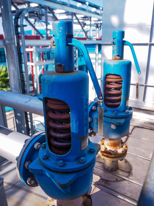
Over the past decade, an increased emphasis on pressure safety valve (PSV) systems has led to increased scrutiny of existing installations in many plants. Often these evaluations uncover gaps between a plant’s existing PSVs and recognized and generally accepted good engineering practice (RAGAGEP). Remedying these issues can lead to costly modifications. One of the most common issues operating companies run into is the 3% rule. Fortunately, new guidance by the American Petroleum Institute (API) on ‘engineering analysis’ allows for operating companies to potentially exceed the 3% rule and avoid costly facility modifications.
What is the 3% rule?
The 3% rule states that the non-recoverable pressure drop in the inlet piping to a PSV should be less than 3% of the valve set pressure. This guideline was developed as a way to ensure PSV stability and prevent valve chatter. Further, PSV relief capacities are based on the stagnation pressure at the nozzle inlet. Inlet losses that exceed 3% cannot be ignored when determining PSV capacity (see 520,II, 7.3.2 ). The 3% rule is cited in various standards, most notably API 520 Pt II and ASME Sec VIII Div I Appendix M. OSHA considers the 3% rule RAGAGEP, and thus it is considered a requirement for installed PSVs. The conventional way to meet the 3% rule for existing installations is through physical modifications such as:
Installing a remote sensing pilot operated relief device or other relief device (such as a rupture disk) that is expected to operate in a stable range with inlet line losses above 3%.
Reduce the capacity of the PSV, such that inlet line losses are reduced. This may be accomplished with a smaller orifice size or a restricted lift.
Installing larger and/or shorter inlet piping to the PSV.
All of the above solutions require physical changes that may require significant capital expense or may not even be feasible for some systems. However, there is another option to consider to potentially avoid these costly modifications.
Engineering Analysis of PSV Stability
API 520 Pt II states that the 3% may be exceeded if “an engineering analysis is performed”. Historically many installations throughout the chemical and refining industries have not followed the 3% rule. In the past, it was not uncommon for operating companies to accept inlet pressure drops up to 5%. For example, one common rule of thumb is to keep PSV inlet line losses below the PSV blowdown percentage, plus some safety factor. This was often considered a sufficient ‘engineering analysis’ to exceed the 3% rule. However, API 521 Pt II has provided more definition on what should be included in an engineering analysis in the latest (7th) edition.
An engineering stability analysis usually consists of qualitative and quantitative assessment. The qualitative assessment typically includes a review of PSV relief history and inspection/repair reports to identify any history of chatter. If a qualitative analysis shows no signs of chatter the quantitative analysis is performed. A quantitative analysis consists of both a force balance and acoustic analysis.
What is a PSV Force Balance?
A PSV force balance is used to determine if a PSV is expected to stay open during a relief event by comparing the sum of forces acting to open the valve against the sum of the forces acting to close the valve. API 520 Part II gives an equation for a conventional PSV force balance as:
Popen – ΔPf,wave – ΔPwave – ΔPbuilt-up > Pclose
Where Popen is the relief pressure, ΔPf,wave is the frictional pressure drop as the PSV is opening, ΔPwave is the recoverable wave line losses, ΔPbuilt-up is the built up backpressure, and Pclose is the reseating pressure. A relief device would ‘pass’ the force balance if the relief pressure minus all of the pressure losses was still greater than the reseating pressure. This indicates that the PSV will stay open even as the pressure wave moves through the inlet piping, indicating that the valve will likely be stable during relief.
Performing an Acoustic Analysis
Suppose that the force balance inequality above is not met? Then the PSV may be expected to reseat during relief, possibly leading to unstable operation. However, an acoustic analysis can determine if the reflection of the pressure wave will reach the PSV inlet before or after the valve closes. To perform an acoustic analysis, a ‘critical’ line length is calculated. A line length near or above the critical line length indicates that instability may occur. API 520 Part II defines the critical line length as follows:
Lcrit = Cto / 2
Where C is the speed of sound, and to is the PSV opening time.
Putting it all together
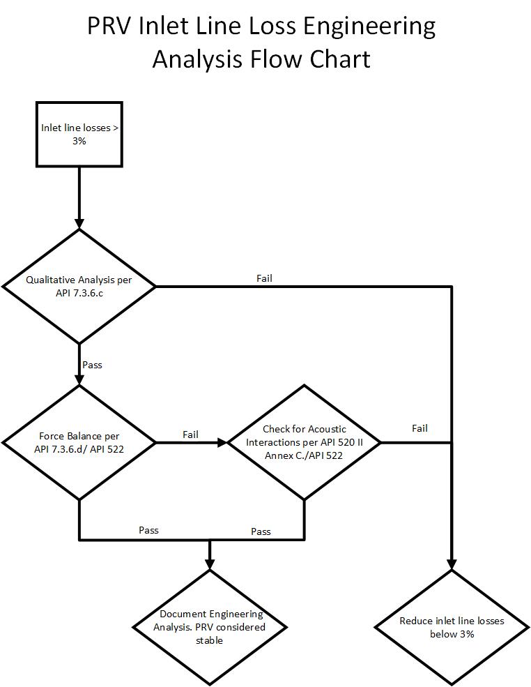
Based on the new API guidelines, an engineering analysis including both a qualitative and quantitative assessment could allow non-recoverable pressure losses in the inlet piping to exceed the 3% using conventional PSVs. The flowchart below outlines the process of performing such an engineering analysis.
By performing these steps, operating companies can avoid costly physical modification to their facilities, while ensuring that they are meeting RAGAGEP guidelines and preventing PSV instability. If you have PSV systems that do not meet the 3% rule, or you are unsure what the inlet pressure drop for your system is, reach out to us at Process Engineering Associates. We have extensive experience with relief system evaluation in a variety of industries. Give us a call to see how we can potentially help you avoid costly modifications and have peace of mind that your PSVs will operate as expected.
References
1. American Society of Mechanical Engineers, ‘Boiler and Pressure Vessel Code, Section VIII, Division I, Rules for the Construction of Pressure Vessels’ (2019).
2. American Petroleum Institute, ‘API Standard 520, Sizing, Selection, and Installation of Pressure-Relieving Devices, Part II – Installation’, 7th edition (2020).
Senior Process Engineer at Process Engineering Associates
March 18, 2024
Background
Various assessments are conducted to promote the safe and reliable operation of process plants in the industry. Some of these assessments include: Hazard and Operability (HAZOP), Process Hazard Analysis (PHA), and Layer of Protection Analysis (LOPA).
During these workshops, a group of cross-functional individuals (often engineers and safety professionals), work together to identify the major hazards within process units. Once these hazards are identified, the team develops effective preventive measures. The identification of such hazards serves as a crucial step in mitigating potential safety and environmental incidents.
Estimating theoretical consequences during a hazards assessment is often done qualitatively. While value can be provided in this manner, it must be noted that other tools exist for a process engineer to support these events in a more quantitative approach. Namely, detailed dispersion modeling. Dispersion modeling can provide numerical results as well as visual graphical representation of the identified consequences. The results from such modeling can be overlaid on plant plot plans or even Google Earth imagery during PHA/HAZOP/LOPA workshops to provide further clarity in evaluating hazardous scenarios. Team members can then further enhance their understanding of an incident by visualizing the impact of the release to the three-dimensional surroundings, such as equipment or buildings.
PROCESS has experience using such modeling tools to support our clients during these assessments.
Practical Examples of Dispersion Modeling
A detailed dispersion modeling effort using well designed software generally allows for a wide range of equipment and consequence scenarios to be evaluated to support these hazard assessments. PROCESS has utilized industry accepted dispersion/modeling tools (i.e. Chemcad, ALOHA, DNV PHAST, etc.) to support clients with their hazard assessments. Some specific examples include: (1) pressure relief device (PRD) atmospheric release dispersion modeling, (2) flare thermal radiation and/or flameout modeling, and (3) In-building chemical releases. Such examples are further discussed as following:
1. Pressure Relief Device Modeling
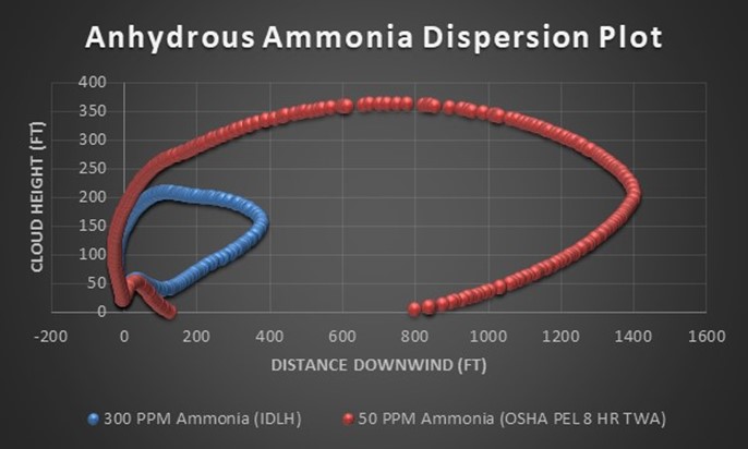
Relief devices that are not connected to a closed relief system (flare header, knock out pot, etc.) should have the tail-pipes directed to a safe relief location. Determining if the atmospheric release is truly to a safe location is a requirement defined by OSHA and ASME. This practice is also recommended in API 520, Part I. Dispersion modeling can provide results to determine relief discharge piping height and location requirements to comply with these codes and standards. PROCESS has conducted various dispersion modeling assessments for clients who wish to understand the potential impacts of a toxic chemical release from a safety valve to the atmosphere. PROCESS recently conducted dispersion modeling on a large anhydrous ammonia storage tank with 3 PRDs (atmospheric relief). The model indicated that during a fire scenario, the atmospheric relief could potentially result in toxic conditions to nearby structures or locations in the plant. Our client used the data from the modeling to support their safety plan.
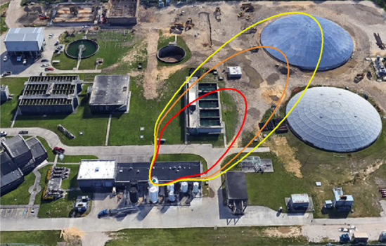
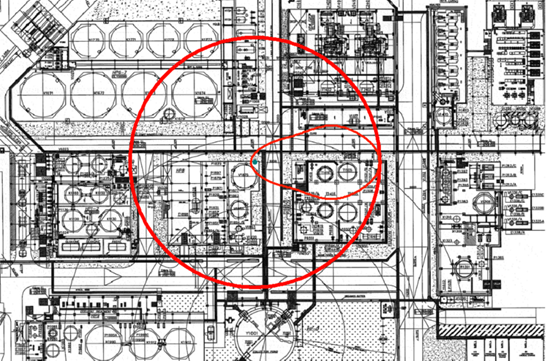
In addition, atmospheric PRD dispersion results can be overlaid on satellite imagery to provide further insight when evaluating hazardous scenarios.
2. Flare Thermal Radiation or Flameout Modeling
Flares provide a certain amount of thermal radiation to nearby pipe racks, buildings, people, and process equipment. This level of radiation changes depending on flaring amount, duration, and certain environmental factors such as wind or time of day. Dispersion modeling can support a project by allowing such radiation effects to be plotted over various radiation levels. This may prove to be beneficial should new equipment, buildings, or pipe racks need to be installed or re-routed.
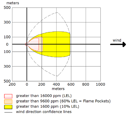
Additionally, during a flare flameout scenario, a large flammable cloud may persist for quite some distance. Dispersion modeling can support the effects of such a scenario. PROCESS has recently conducted a similar exercise for a client who was considering a hypothetical large hydrocarbon release occurring while the pilots were distinguished on the flare. Dispersion modeling for that exercise revealed where flammable regions may exist on the site plot plan.
3. Inside Building Releases
Inside building releases can be modeled. For example, an indoor leak in a lab may build up a large concentration prior to being released outside. The outdoor release and effects can be modeled, along with possible explosion effects.
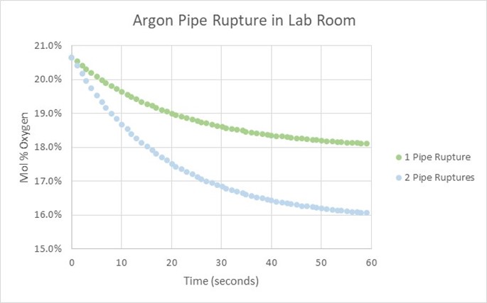
In addition, indoor releases can be modeled considering asphyxiation, by showing oxygen depletion over-time at certain portions in a room or building. This may be valuable if there is a need to consider a nitrogen or argon line rupture in an occupied room. PROCESS has conducted such an exercise for a client with a lab environment where an argon pipe rupture was considered. The room oxygen concentration was estimated over time as the leak event unfolded. This helped the client determine safety planning if such an incident should unfold.
Other Potential Uses for Dispersion Modeling
While a few practical examples were listed, dispersion modeling may also prove to add value for various other incidents or planning efforts. These include, but are not limited to:
Emergency Response Planning
Incident investigation
Spill and Loss of Containment Events
Pipeline Leaks
Facility Citing and Occupied Building Risk Assessments
Conclusion
Whether the end user is in oil and gas, petrochemical, pharmaceutical, the public sector, or a storage facility; accurate dispersion modeling can be an important tool to help ensure safety is not compromised during the design and operation of a facility.
A detailed dispersion study can provide numerical and visual representation of potential consequences identified in hazard assessments (e.g. PRD relief, flare upset condition, inbuilding rupture releases, etc.). Such results allow safety professionals to develop strategies to prevent future re-occurrences, develop best practices, and make informed decisions to emergency response plans and overall safety measures.
References
1. American Society of Mechanical Engineers, ‘Boiler and Pressure Vessel Code, Section VIII, Division I, Subsection A, Part UG-135(f) (2009).
2. Occupational Safety and Health Administration (OSHA), 1910 Subpart H, Hazardous Materials, Dispensing Devices, 1910.110(h)
3. American Petroleum Institute, API 520, Part I, 10th Ed. (2020), Section 4 – Pressure Relief Devices
PROCESSis pleased to announce that Matt Whitworth, working out of the Oak Ridge, Tennessee office, has just recently completed the requirements for and been awarded his P.E. license for the state of Tennessee. We congratulate Matt on achieving this significant accomplishment. Matt is the technical lead for the Industrial Services Group in the Tennessee office.
PROCESS is also please to announce that Chris Muntean, P.E. as part of his continuing education and working out of the Oak Ridge, Tennessee office, has just recently completed the requirements for and been awarded his certificate for completing ELP303: RAPID’s Process Intensification Credential Program with a focus on heat and mass transfer. This course was offered through the AIChE Academy.
Matt is currently a Chief Process Engineer, a chemical engineer (B.S., Georgia Institute of Technology, 1998) with 23 years experience in the design, startup, and operation of batch and continuous organic chemical production processes, alternative energy process design, as well as in computer process modeling and simulation and Six Sigma methodologies.
Chris is currently a Senior Process Engineer, a chemical engineer (B.S., University of Toledo, 2006) with 17 years experience in the design, commissioning, startup, and operation of continuous chemical production processes, process design project management, project engineering, control system programming, as well as in computer process modeling and simulation and management of change.
We congratulate both Matt and Chris on achieving these significant accomplishments!
Process Engineer at Process Engineering Associates
October 24, 2020
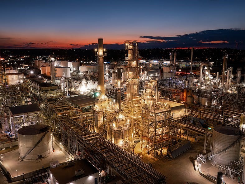
Due to the current economic climate, many refineries and petrochemical plants are running at reduced capacities. Operating companies are more closely scrutinizing operating expenses in this low margin environment. As a process engineer or operations professional, we have the opportunity to find ways to reduce operating expenses by reducing energy consumption.
One of the areas inside process plants that takes up significant energy is distillation and fractionation. Distillation consumes over 40% of the total energy in the refining and chemical industry(1). In fact, distillation is 6% of the total energy usage in the United States. This is an incredible amount of energy! Thus process engineers should be consistently asking, am I minimizing energy usage in my distillation columns?
Two ways to reduce distillation energy usage are eliminate excess reflux and reduce tower pressure.
Is Your Distillation Column Over-refluxed?
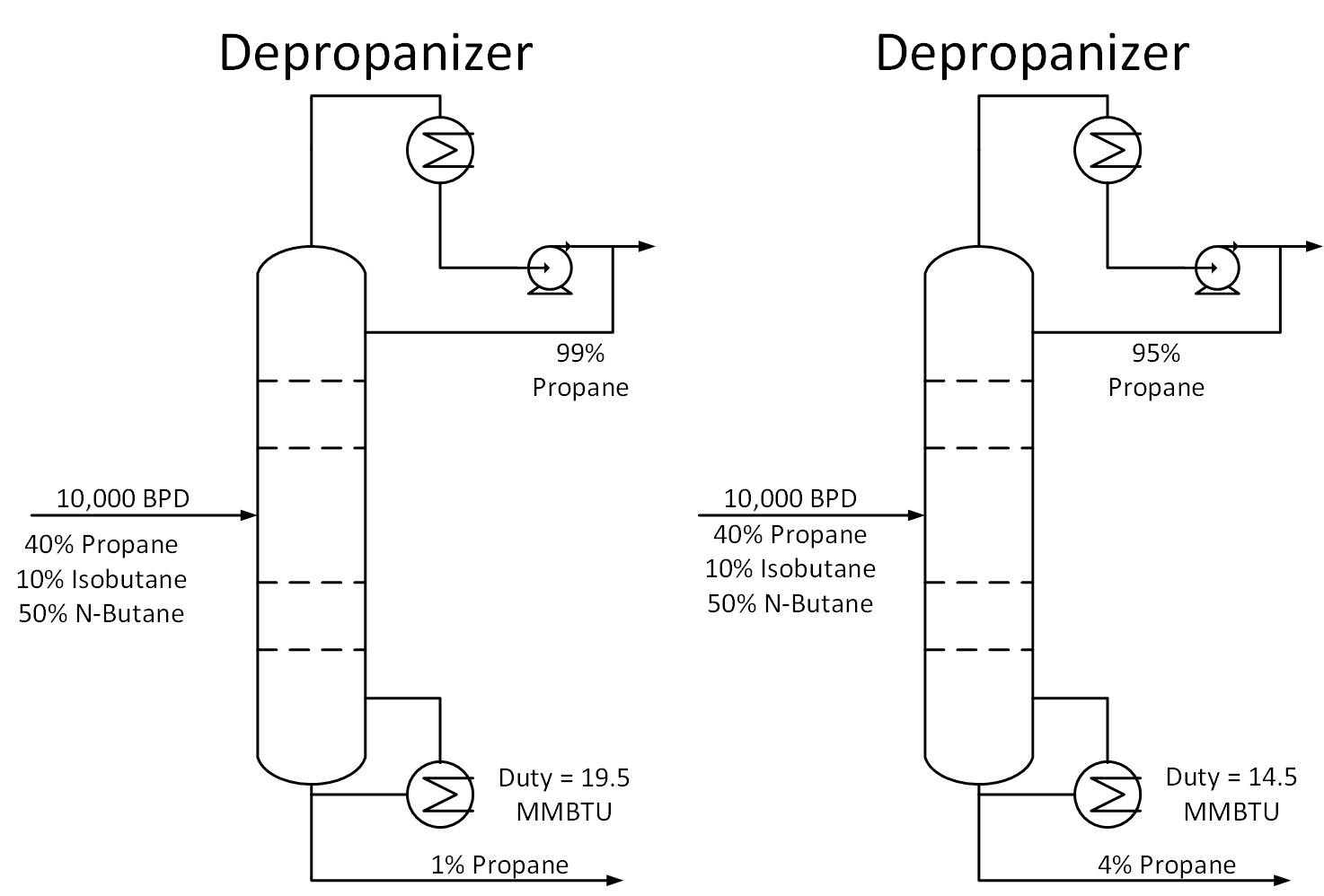
Is your distillation column over-refluxed? To answer this question, determine the specifications required for each stream exiting a column. For example, a depropanizer column in a refinery may require a 95% propane product purity and at least 95% butane concentration in the bottoms stream. Suppose the column is operating at 99% propane purity while meeting bottoms specifications. How much energy is being wasted in this scenario?
The figure below shows the difference in duty for the two cases described above. The 99% purity case consumes 33% more energy than the 95% purity case. For the 10,000 BPD example below, this translates to a savings of 5 MMBTU/HR. If energy in this scenario costs $3/MMBTU, this would come out to $130K per year in energy savings.
Typically operators will target above the required product purity to absorb any swings in tower operation while keeping product streams on spec. Reducing this ‘overshoot’ as much as feasible can result in great energy savings.
Over refluxing towers wastes a significant amount of energy, and sometimes with little or unnecessary improvement in product purity or yields.
Reducing Energy Usage by Decreasing Operating Pressure
Another way to reduce energy usage is by reducing tower pressure. This can be especially effective in the winter months, when cooling water and ambient temperatures are lower, increasing the available process cooling. Reducing tower pressure reduces energy consumption because the relative volatility of hydrocarbons increases at lower temperatures. This makes them easier to separate, i.e. requiring less energy. This is especially true of lighter hydrocarbons (C1-C6).
The Cox Diagram(3) above shows why decreasing column pressure reduces energy consumption. For any given compound, as column pressure decreases, the flash temperature also decreases. The diagram above shows the relationship between flash temperature and vapor pressure. As flash temperature decreases, so does the vapor pressure for each hydrocarbon. But more importantly, the difference in vapor pressure between the compounds increases. For example at 180 deg F, The relative volatility between propane and butane is
Relative Volatility @ 180 F= VP C3/ VP C4
= 400 psig/150 psig
= 2.7
Suppose the overhead pressure in a column is lowered until the overhead temperature reaches 100 deg F.
Relative Volatility @ 100 F= VP C3/ VP C4
= 200 psig/ 50 psig
= 4.0
As shown above, decreasing operating pressure will increase relative volatility. This in turn reduces the required energy to perform a given separation. Let’s return to our depropanizer example. Suppose we drop the operating pressure in this tower from 300 psig to 275 psig. This reduces the required energy in our tower by 7%, saving $25k/year in our example.
One thing to consider when reducing tower pressure is that the reduction in tower pressure will cause an increase in vapor velocity inside the tower. This increases the chance of flooding inside the tower.
Savings energy is not only good for the bottom line, it is also good for the environment, conserving natural resources. If you find this article useful, let me know in the comments below. What ways have you reduced energy usage in distillation columns?
Process Engineer at Process Engineering Associates
_____________
Recently I saw a safety article that resonated with me. The topic, Trusting Plant Instruments.
Few days go by where myself or a coworker don’t question an instrument reading at the plant I work at. And how could you not? Everyday, process engineers and operations personnel are looking at dozens or hundreds of instrument outputs. And every so often, we come across a reading that doesn’t make sense. But how operation personnel respond to an instrument that “doesn’t make sense” can have serious process safety implications.
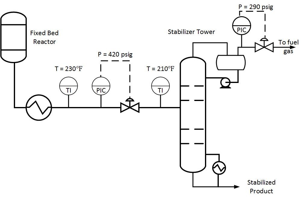
I had an experience that made this principle quite clear to me. The process flow diagram below shows the process I was working with.
I was helping with the start up of a new bypass around an exchanger. We were monitoring the feed temperature to the stabilizer tower. If the stabilizer feed temperature got too high, liquid traffic in the stripping section of the tower would be reduced, and stripping efficiency would suffer. Our goal was to keep the feed temperature at the design value of 215 deg F.
As shown above, the unit described above has two feed temperature indications. But one was reading above the design value, and one was below. So then, which one is correct? Both values can not be correct, as there is no heat exchange occurring between the temperature indications.
I looked through the process graphics and trends, self-assured that I would determine which instrument was faulty. But in my search to justify my own assumptions, I realized something unexpected, both instruments were correct.
How can this be? Well dear reader, if you study the process flow diagram above, you will notice a control valve between the two thermocouples. A small portion of the stream flashed as it flowed through the control valve, cooling the stream before it entered the tower. Indeed, both thermocouples were correct!
So why am I telling this story? I believe it teaches a valuable concept. I didn’t understand how both instruments could be correct, so I immediately assumed one reading was false. This is the wrong way to think about instrument readings. When plant personnel ignore instrumentation, it is often because we don’t understand how the reading is possible. We then discard the reading as erroneous to justify our own notions of what is occurring inside our processes. This can lead to serious process safety implications, as the two examples below show.
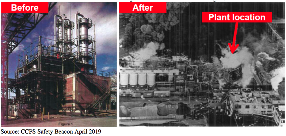
In the 1960’s, a fire and explosion occurred chemical plant in Tennessee during a unit start-up (1). a thermocouple inside a distillation column was reading 250 degrees when it “should have” read 215 degrees. An instrument technician was sent into the unit to troubleshoot the instrument just before the explosion. A post-incident investigation revealed that the high temperature readings were consistent with increased Nitrobenzene content on that tray, likely due to tray damage. Had plant personnel not ignored this information, the incident may have been avoided.
Before and after of a Tennessee chemical plant fire
Another incident occurred in the 1990’s at a California Oil Refinery (2). A hydrocracker reactor outlet temperature went off-scale high, indicating a run away reaction. The control board operator was hesitant to believe the temperature reading, and did not depressure the reactor to stop the reaction. The ensuing fire and explosion resulted in one fatality and 46 injuries.
Not trusting process instrumentation can lead serious incidents. This is especially true for instruments that indicate an unsafe condition. So what can you do to make sure this doesn’t happen to you?
Assume an instrument is working until proven otherwise, especially when the reading could indicate an unsafe process condition. Ask yourself, What are the consequences if this instrument is reading correctly? Then take appropriate action.
Use other instruments and samples to confirm suspicious readings.
And finally, don’t assume an instrument isn’t working because you don’t understand how the reading could be correct!
Sources
Center for Chemical Process Safety April 2019 Safety Beacon EPA Chemical Accident Investigation Report Tosco Avon Refinery, Martinez, California
Calumet Specialty Products Partners LP is a long-time client of Process Engineering Associates, LLC (PROCESS). Their subsidiary company, Montana Renewables, recently achieved design throughput capacity for processing renewable feedstocks into low-emission sustainable fuel alternatives at the operator’s renewables manufacturing plant in Montana.
Calumet Specialty Products Partners LP subsidiary Montana Renewables LLC (MRL) has achieved the design throughput capacity for processing renewable feedstocks into low-emission sustainable fuel alternatives at the operator’s renewables manufacturing plant in Great Falls, Mont. (read the full story here: OGJ Online, Sept. 8, 2021).
Co-located at fellow subsidiary Calumet Montana Refining LLC’s (CMRL) Great Falls conventional refinery and specialty asphalt plant, MRL’s biorefinery reached its design processing capacity for renewable feedstocks of 15,000 b/sd as of Apr. 18 following commissioning of the operator’s new renewable hydrogen plant on Mar. 4, Calumet said.
While Calumet did not disclose a capacity of the new hydrogen plant, the new installation produces renewable hydrogen—or green hydrogen—by splitting water into hydrogen and oxygen using hydrogen gases collected from the biorefinery’s renewable diesel reactor. The plant then recycles the green hydrogen for reuse within the biorefinery using a patent-pending but yet-to-be-identified technology, according to MRL’s website.
PROCESS congratulates Calumet Montana Refining on this very significant accomplishment and wishes them many productive, profitable, and safe years of operation to come.


 Typically operators will target above the required product purity to absorb any swings in tower operation while keeping product streams on spec. Reducing this ‘overshoot’ as much as feasible can result in great energy savings.
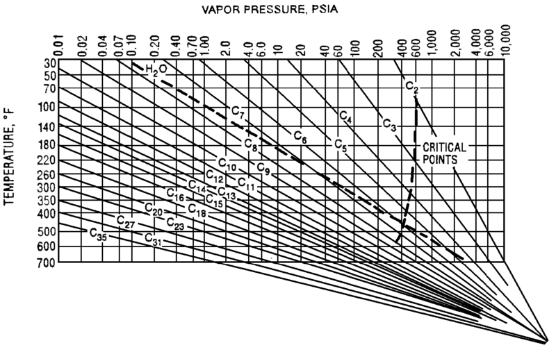 The Cox Diagram(3) above shows why decreasing column pressure reduces energy consumption. For any given compound, as column pressure decreases, the flash temperature also decreases. The diagram above shows the relationship between flash temperature and vapor pressure. As flash temperature decreases, so does the vapor pressure for each hydrocarbon. But more importantly, the difference in vapor pressure between the compounds increases. For example at 180 deg F, The relative volatility between propane and butane is
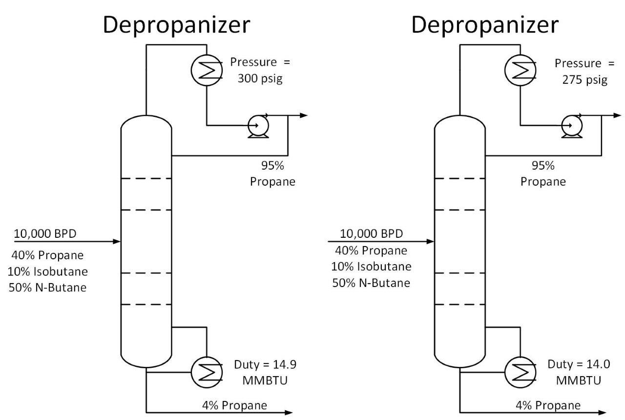 One thing to consider when reducing tower pressure is that the reduction in tower pressure will cause an increase in vapor velocity inside the tower. This increases the chance of flooding inside the tower.