Category: Blog

A Look Inside a Process Engineer’s Toolbox: Dispersion Modeling


Written by: Christopher J. Muntean, P.E.

Senior Process Engineer at Process Engineering Associates

March 18, 2024


Background

Various assessments are conducted to promote the safe and reliable operation of process plants in the industry. Some of these assessments include: Hazard and Operability (HAZOP), Process Hazard Analysis (PHA), and Layer of Protection Analysis (LOPA).

During these workshops, a group of cross-functional individuals (often engineers and safety professionals), work together to identify the major hazards within process units. Once these hazards are identified, the team develops effective preventive measures. The identification of such hazards serves as a crucial step in mitigating potential safety and environmental incidents.

Estimating theoretical consequences during a hazards assessment is often done qualitatively. While value can be provided in this manner, it must be noted that other tools exist for a process engineer to support these events in a more quantitative approach. Namely, detailed dispersion modeling. Dispersion modeling can provide numerical results as well as visual graphical representation of the identified consequences.  The results from such modeling can be overlaid on plant plot plans or even Google Earth imagery during PHA/HAZOP/LOPA workshops to provide further clarity in evaluating hazardous scenarios.  Team members can then further enhance their understanding of an incident by visualizing the impact of the release to the three-dimensional surroundings, such as equipment or buildings.

PROCESS has experience using such modeling tools to support our clients during these assessments.

Practical Examples of Dispersion Modeling

A detailed dispersion modeling effort using well designed software generally allows for a wide range of equipment and consequence scenarios to be evaluated to support these hazard assessments. PROCESS has utilized industry accepted dispersion/modeling tools (i.e. Chemcad, ALOHA, DNV PHAST, etc.) to support clients with their hazard assessments. Some specific examples include: (1) pressure relief device (PRD) atmospheric release dispersion modeling, (2) flare thermal radiation and/or flameout modeling, and (3) In-building chemical releases. Such examples are further discussed as following:

1. Pressure Relief Device Modeling

Relief devices that are not connected to a closed relief system (flare header, knock out pot, etc.) should have the tail-pipes directed to a safe relief location. Determining if the atmospheric release is truly to a safe location is a requirement defined by OSHA and ASME. This practice is also recommended in API 520, Part I. Dispersion modeling can provide results to determine relief discharge piping height and location requirements to comply with these codes and standards. PROCESS has conducted various dispersion modeling assessments for clients who wish to understand the potential impacts of a toxic chemical release from a safety valve to the atmosphere.  PROCESS recently conducted dispersion modeling on a large anhydrous ammonia storage tank with 3 PRDs (atmospheric relief). The model indicated that during a fire scenario, the atmospheric relief could potentially result in toxic  conditions to nearby structures or locations in the plant. Our client used the data from the modeling to support their safety plan.

In addition, atmospheric PRD dispersion results can be overlaid on satellite imagery to provide further insight when evaluating hazardous scenarios.


2. Flare Thermal Radiation or Flameout Modeling

Flares provide a certain amount of thermal radiation to nearby pipe racks, buildings, people, and process equipment. This level of radiation changes depending on flaring amount, duration, and certain environmental factors such as wind or time of day. Dispersion modeling can support a project by allowing such radiation effects to be plotted over various radiation levels. This may prove to be beneficial should new equipment, buildings, or pipe racks need to be installed or re-routed.

Additionally, during a flare flameout scenario, a large flammable cloud may persist for quite some distance. Dispersion modeling can support the effects of such a scenario.  PROCESS has recently conducted a similar exercise for a client who was considering a hypothetical large hydrocarbon release occurring while the pilots were distinguished on the flare. Dispersion modeling for that exercise revealed where flammable regions may exist on the site plot plan.

3. Inside Building Releases

Inside building releases can be modeled. For example, an indoor leak in a lab may build up a large concentration prior to being released outside. The outdoor release and effects can be modeled, along with possible explosion effects.

In addition, indoor releases can be modeled considering asphyxiation, by showing oxygen depletion over-time at certain portions in a room or building. This may be valuable if there is a need  to consider a nitrogen or argon line rupture in an occupied room. PROCESS has conducted such an exercise for a client with a lab environment where an argon pipe rupture was considered. The room oxygen concentration was estimated over time as the leak event unfolded. This helped the client determine safety planning if such an incident should unfold.

Other Potential Uses for Dispersion Modeling

While a few practical examples were listed, dispersion modeling may also prove to add value for various other incidents or planning efforts. These include, but are not limited to:

  • Emergency Response Planning
  • Incident investigation
  • Spill and Loss of Containment Events
  • Pipeline Leaks
  • Facility Citing and Occupied Building Risk Assessments


Conclusion

Whether the end user is in oil and gas, petrochemical, pharmaceutical, the public sector, or a storage facility; accurate dispersion modeling can be an important tool to help ensure safety is not compromised during the design and operation of a facility.

A detailed dispersion study can provide numerical and visual representation of potential consequences identified in hazard assessments (e.g. PRD relief, flare upset condition, inbuilding rupture releases, etc.).  Such results allow safety professionals to develop strategies to prevent future re-occurrences, develop best practices, and make informed decisions to emergency response plans and overall safety measures.

References

1. American Society of Mechanical Engineers, ‘Boiler and Pressure Vessel Code, Section VIII, Division I, Subsection A, Part UG-135(f) (2009).

2. Occupational Safety and Health Administration (OSHA), 1910 Subpart H, Hazardous Materials, Dispensing Devices, 1910.110(h)

3. American Petroleum Institute, API 520, Part I, 10th Ed. (2020), Section 4 – Pressure Relief Devices

Are you minimizing energy usage in your distillation columns?


Written by: Jackson Udy, PE

Process Engineer at Process Engineering Associates

October 24, 2020


Due to the current economic climate, many refineries and petrochemical plants are running at reduced capacities. Operating companies are more closely scrutinizing operating expenses in this low margin environment. As a process engineer or operations professional, we have the opportunity to find ways to reduce operating expenses by reducing energy consumption.

One of the areas inside process plants that takes up significant energy is distillation and fractionation. Distillation consumes over 40% of the total energy in the refining and chemical industry(1). In fact, distillation is 6% of the total energy usage in the United States. This is an incredible amount of energy! Thus process engineers should be consistently asking, am I minimizing energy usage in my distillation columns?

Two ways to reduce distillation energy usage are eliminate excess reflux and reduce tower pressure.

Is Your Distillation Column Over-refluxed?

Is your distillation column over-refluxed? To answer this question, determine the specifications required for each stream exiting a column. For example, a depropanizer column in a refinery may require a 95% propane product purity and at least 95% butane concentration in the bottoms stream. Suppose the column is operating at 99% propane purity while meeting bottoms specifications. How much energy is being wasted in this scenario?

The figure below shows the difference in duty for the two cases described above. The 99% purity case consumes 33% more energy than the 95% purity case. For the 10,000 BPD example below, this translates to a savings of 5 MMBTU/HR. If energy in this scenario costs $3/MMBTU, this would come out to $130K per year in energy savings.


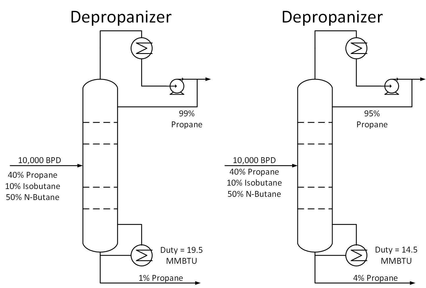
Typically operators will target above the required product purity to absorb any swings in tower operation while keeping product streams on spec. Reducing this ‘overshoot’ as much as feasible can result in great energy savings.

Over refluxing towers wastes a significant amount of energy, and sometimes with little or unnecessary improvement in product purity or yields.

Reducing Energy Usage by Decreasing Operating Pressure

Another way to reduce energy usage is by reducing tower pressure. This can be especially effective in the winter months, when cooling water and ambient temperatures are lower, increasing the available process cooling. Reducing tower pressure reduces energy consumption because the relative volatility of hydrocarbons increases at lower temperatures. This makes them easier to separate, i.e. requiring less energy. This is especially true of lighter hydrocarbons (C1-C6).

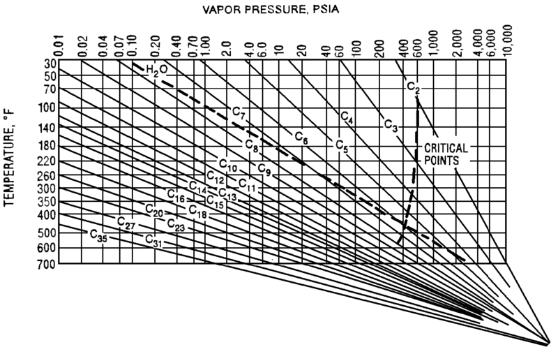
The Cox Diagram(3) above shows why decreasing column pressure reduces energy consumption. For any given compound, as column pressure decreases, the flash temperature also decreases. The diagram above shows the relationship between flash temperature and vapor pressure. As flash temperature decreases, so does the vapor pressure for each hydrocarbon. But more importantly, the difference in vapor pressure between the compounds increases. For example at 180 deg F, The relative volatility between propane and butane is

Relative Volatility @ 180 F= VP C3/ VP C4
= 400 psig/150 psig
= 2.7

Suppose the overhead pressure in a column is lowered until the overhead temperature reaches 100 deg F.

Relative Volatility @ 100 F= VP C3/ VP C4
= 200 psig/ 50 psig
= 4.0

As shown above, decreasing operating pressure will increase relative volatility. This in turn reduces the required energy to perform a given separation. Let’s return to our depropanizer example. Suppose we drop the operating pressure in this tower from 300 psig to 275 psig. This reduces the required energy in our tower by 7%, saving $25k/year in our example.

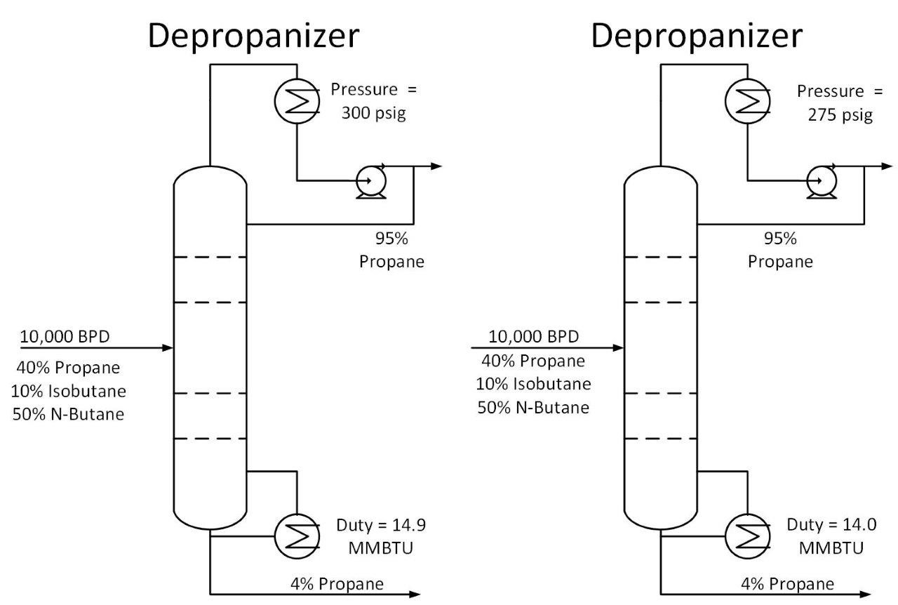
One thing to consider when reducing tower pressure is that the reduction in tower pressure will cause an increase in vapor velocity inside the tower. This increases the chance of flooding inside the tower.

Savings energy is not only good for the bottom line, it is also good for the environment, conserving natural resources. If you find this article useful, let me know in the comments below. What ways have you reduced energy usage in distillation columns?

References

1) https://www.emersonautomationexperts.com/2010/industry/downstream-hydrocarbons/reducing_distil/#:~:text=Did%20you%20know%20that%20there,energy%20consumed%20by%20U.S.%20manufacturers.

2) Lieberman, Norman and Elizabeth Lieberman. A Working Guide to Process Equipment. McGraw-Hill Education, 2014.

3) https://petrowiki.org/Vapor_pressure

Do You Trust Your Process Instruments?

Jackson Udy, PE

Process Engineer at Process Engineering Associates
_____________

Recently I saw a safety article that resonated with me. The topic, Trusting Plant Instruments.

Few days go by where myself or a coworker don’t question an instrument reading at the plant I work at. And how could you not? Everyday, process engineers and operations personnel are looking at dozens or hundreds of instrument outputs. And every so often, we come across a reading that doesn’t make sense. But how operation personnel respond to an instrument that “doesn’t make sense” can have serious process safety implications.

I had an experience that made this principle quite clear to me. The process flow diagram below shows the process I was working with.

I was helping with the start up of a new bypass around an exchanger. We were monitoring the feed temperature to the stabilizer tower. If the stabilizer feed temperature got too high, liquid traffic in the stripping section of the tower would be reduced, and stripping efficiency would suffer. Our goal was to keep the feed temperature at the design value of 215 deg F.

As shown above, the unit described above has two feed temperature indications. But one was reading above the design value, and one was below. So then, which one is correct? Both values can not be correct, as there is no heat exchange occurring between the temperature indications.

I looked through the process graphics and trends, self-assured that I would determine which instrument was faulty. But in my search to justify my own assumptions, I realized something unexpected, both instruments were correct.

How can this be? Well dear reader, if you study the process flow diagram above, you will notice a control valve between the two thermocouples. A small portion of the stream flashed as it flowed through the control valve, cooling the stream before it entered the tower. Indeed, both thermocouples were correct!

So why am I telling this story? I believe it teaches a valuable concept. I didn’t understand how both instruments could be correct, so I immediately assumed one reading was false. This is the wrong way to think about instrument readings. When plant personnel ignore instrumentation, it is often because we don’t understand how the reading is possible. We then discard the reading as erroneous to justify our own notions of what is occurring inside our processes. This can lead to serious process safety implications, as the two examples below show.

In the 1960’s, a fire and explosion occurred chemical plant in Tennessee during a unit start-up (1). a thermocouple inside a distillation column was reading 250 degrees when it “should have” read 215 degrees. An instrument technician was sent into the unit to troubleshoot the instrument just before the explosion. A post-incident investigation revealed that the high temperature readings were consistent with increased Nitrobenzene content on that tray, likely due to tray damage. Had plant personnel not ignored this information, the incident may have been avoided.


Before and after of a Tennessee chemical plant fire

Another incident occurred in the 1990’s at a California Oil Refinery (2). A hydrocracker reactor outlet temperature went off-scale high, indicating a run away reaction. The control board operator was hesitant to believe the temperature reading, and did not depressure the reactor to stop the reaction. The ensuing fire and explosion resulted in one fatality and 46 injuries.

Not trusting process instrumentation can lead serious incidents. This is especially true for instruments that indicate an unsafe condition. So what can you do to make sure this doesn’t happen to you?

  1. Assume an instrument is working until proven otherwise, especially when the reading could indicate an unsafe process condition. Ask yourself, What are the consequences if this instrument is reading correctly? Then take appropriate action.
  2. Use other instruments and samples to confirm suspicious readings.
  3. And finally, don’t assume an instrument isn’t working because you don’t understand how the reading could be correct!

Sources

Center for Chemical Process Safety April 2019 Safety Beacon
EPA Chemical Accident Investigation Report Tosco Avon Refinery, Martinez, California

Limitations of Particle Disengagement Estimation Methods

written by Michael Tanzio, Process Engineering Associates, LLC; February 2021

The industrial literature is full of stories about poor separation in systems consisting of drops or particles in a separate continuous phase (gas or liquid).  Poor disengagement of the dispersed phase can lead to major, unwanted, economic consequences (poor product quality, reduced throughput, environmental and safety consequences, plugged piping, damaged equipment, etc.). Many times, this poor performance can be traced to the following:

  • Use of poor design methods for sizing the separation vessel
  • Lack of complete and valid information on the system (volume fraction of dispersed phase, particle size distribution, particle shape and density, etc.).

But how do you know a design method is poor? Or what data and information is required for a high-quality design? These can be answered, in part, by understanding the assumptions and limitations inherent in the design method being used. If the assumptions and limitations for the system is within those of the design method, then your design is probably working. If not, then you are probably reaching for your wallet!

For this discussion “particle” refers to both solid particles and liquid drop particles.

The majority of disengagement calculation methods are limited by the following assumptions inherent in the calculations:

  • The particles are rigid, undistorted spheres.
  • The drag force is the major force contributing to momentum exchange between the phases. Particle rotation (Magnus lift force), gradient forces (concentration, velocity (Saffman force), pressure, temperature), virtual mass effects, Basset force effects, collisional forces, electrostatics, all friction, viscous stress and turbulent stress are neglected (references 15, 16).
  • The fluid system is dilute with the particles existing at very low volume fractions in the total fluid.
  • The continuous phase is a quiescent fluid and relative velocity is negligible.
  • The particles are not hindered in their settling by other particles.
  • Dispersion bands are not considered.
  • The fluids are Newtonian.
  • The particles are larger than the mean free path of the continuous gas phase and Brownian motion is not important.
  • Wall effects on particle settling are negligible.
  • There are no phase changes or mass transfer occurring in the vessel.

A number of other assumptions also limit the use of many design methods. The ones listed above are considered the major factors limiting current design methods.

Although these assumptions should satisfy the majority of the systems analyzed, there may be cases where these assumptions are not valid. A qualitative discussion of some of these effects is presented next with some guidance on when they should be considered. References are also cited for further information.

Particle Distortion

The equations used to estimate terminal velocity are for rigid, spherical particles in a stagnant medium. However, liquid drops in motion may not be rigid or spherical. Up to a certain transition drop size, the terminal velocity can be higher than estimated due to internal circulation within the drop. As the drop size increases, a transition point is reached where the drop starts to oscillate and distort from a spherical shape. At this transition, the terminal velocity is a maximum and starts to decrease as the drop size gets larger.

Complicating the phenomena are the effects that contaminants or surfactants may have on the internal circulation and drop distortion. The demarcation between a spherical particle and a distorted particle is a function of both the Eotvos (Eo) number and particle Reynolds (Re) number. Below a particle Re of about 1.2, particles should remain spherical at all Eo numbers. At Eo numbers greater than about 0.4, particle distortion may be important. Either the Clift correlation (References 1 and 2) or the Hu & Kintner correlation (Reference 3) can be used to estimate the effect of particle distortion.

Dilution and Hindered Settling

The majority of design methods assume the concentration of drops in the dispersed phase is very low. These methods are probably valid only for dispersed phase volumetric hold-ups below 0.03 in the Stoke’s regime and below 0.05 in the Newton regime. This is due to two factors:

  1. As a design requirement, many current design methods set the maximum superficial velocity of the continuous phase to be equal to the terminal velocity of a single particle in a stagnant fluid. However, the real velocity of the continuous phase is the proper velocity to use, and, in a moving fluid, the drag force depends on the relative velocity between the drops and the continuous phase. In a multiphase system, when the drag force balances the gravity and buoyancy forces, the resulting velocity is the relative velocity between the phases.

But most methods assume the resulting velocity is the terminal velocity of the dispersed phase in a stagnant fluid. A particular terminal velocity applies only to one particle diameter. By making the continuous phase velocity equal to the terminal velocity, all particles having that terminal velocity will not move or settle out. If particles and drops having only that particle diameter exist in the system, nothing gets separated until solid particles collide or liquid drops coalesce.

  • At high dispersed phase hold-ups, dispersed phase settling becomes hindered and the terminal velocity is significantly reduced. Unlike hindered solid settling, as the dispersed phase hold-up increases, drop coalescence becomes more important. At some point coalescence starts affecting the drag force on the drop. Initially, at low coalescence rates, the terminal velocity decreases due to the hindering by other drops.  As coalescence becomes more important, the terminal relative velocity starts to increase and dominates the hindering effect.

For solid particles, unless they stick together, no such coalescence occurs. The terminal velocity is then reduced and the solid particles become entrained in the continuous phase.

In the design of many systems, these effects are usually ignored. Either a conservative, effective, design particle diameter or a disengagement “K” value is used. The K-value method (reference 17) estimates the required continuous phase velocity to be used for design.

The design particle diameter and / or K-value is based on past experience. Although providing a workable design, the use of these methods can be very conservative, or they can provide for an unworkable design.

What if a design value for a particular system is not known? Guidance on design values are available only for a relatively small number of industrially significant systems. If a system deviates from these “norms”, then the dispersed phase hold-up, and the real particle diameter to be disengaged, needs to be known. A rough estimate of the dispersed phase hold-up can be made by assuming a homogeneous flow regime similar to vapor/liquid, two-phase pipe flow system analysis. The hold-up is then just the fraction of the total volume that is the dispersed phase.

However, if significant slip between the phases occurs, the homogeneous hold-up may not be correct. Relatively small changes in the dispersed phase hold-up can result in large changes in the dispersed phase settling velocity with ramifications for vessel sizes. For example, past experience (Reference 4) on a liquid/liquid system showed the ratio of dispersed phase velocity to that of a single particle to be about 0.7 at a dispersed phase hold-up of only 0.05 and about 0.5 at a hold-up of only 0.1.

If the homogeneous hold-up is greater than about 0.03, then experimental measurement of the actual hold-up needs to be considered.

The determination of solid particle diameters is relatively easy compared to that of liquid drops. Liquid drop diameters are difficult to estimate since they depend on the upstream process history of the fluid entering a vessel. It is well known that drop size within a system is inversely proportional to the energy dissipated per unit mass in that system. Therefore, upstream equipment with high energy input (agitators, pumps, etc.) or with high energy losses (high pressure drop control valves, pipe frictional losses, etc.) will tend to produce drops with small diameters. Various correlations are available to estimate drop sizes but they should be used with caution. Further information on drop size estimates can be found in References 5, 6, 7, and 8. Agreement by the client for the drop size estimated and to be used for vessel design is imperative. Note that this must be a true diameter and not an effective design diameter. 

Once particle hold-up and diameter are known, the terminal velocity for a single particle in a stagnant media can be corrected to account for the presence of multiparticles. A number of methods are available:

  • Ishii and Zuber (reference 9) developed drag coefficient and relative motion correlations from simple similarity criteria and a mixture viscosity model. They showed that the drag law for dispersed two-phase flows of bubbles, drops and particles could be put on a general and unified basis. Their unified method also accounts for the distortion of bubbles and drops.
  • A Richardson / Zaki type of correlation as presented by Maude & Whitmore is described in references 3 and 10.
  • The Zenz correlation for particulate fluidization (reference 11) can be used to directly estimate the relative velocity. The use of Zenz’s correlation to adequately determine the relative velocity in a counterflow, spray tower extractor is described in an older edition of Perry’s (reference 12). Note that much of the data Zenz used for his correlation was based on sedimentation data.
  • The continuous phase superficial velocity can be estimated for vertical liquid/liquid separators directly from the extractor flooding correlation of Minard and Johnson (reference 13). The design velocity can be chosen at about 40 percent of the flood velocity.
  • Rietema discusses other correlations in his review article (reference 14). This article is also an excellent discussion of dispersed two-phase systems.

None of these methods have been evaluated or compared. They are offered as starting references. Applicability to the particular system being analyzed should be determined.

As the dispersed phase hold-up approaches 0.2 to 0.3, drop coalescence effects may become important. Larger drops form due to the “crowding” caused by the high dispersed phase volume fraction. This author does not know of any current method for determining these coalescence effects.  Reader suggestions are welcomed. However, a workable, conservative design can be obtained by neglecting coalescence and using a smaller particle size. For hold-ups of this magnitude, two separators may be required: one to knock-out the bulk of the dispersed phase and a secondary one for removal of the smaller particles.

Dispersion Bands

Liquid / liquid gravity separator performance depends on two phenomena:

  1. the movement of drops to the liquid / liquid interface;
  2. the coalescence of drops at the interface.

Liquid drops crossing the interface can form a deep band of dispersed drops (reference 7). Many design methods do not allocate vessel volume for a liquid dispersion band. They usually assume, for a liquid/liquid system, a dilute system and a conservative, effective drop diameter for design. This combination may provide enough volume for any dispersion band that may actually develop. But I have seen no data to confirm that. It is prudent to base the design on the actual, measured dispersed phase hold-up and the real, measured drop diameter. Adequate volume needs to be provided for a dispersion band. But if the band height is a significant fraction of the separator depth, a small increase in feed rate could flood the separator with the dispersion band resulting in poor, or no, liquid / liquid separation.

Davies (reference 5) presents a correlation for estimating the time required for coalescence of drops in a multi-drop system. Reference 7 provides some design criteria for determining the dispersion band volume.

Other Limitations

Other major assumptions are that the fluids are Newtonian and the drop sizes are above 2 mm. Perry’s (Reference 1) provides some guidance on non-Newtonian fluids. For small drops in a gas, the size can become comparable to the mean free path of the gas. Below about 2 mm in diameter, the terminal velocity of a drop in a gas needs to be corrected by applying the Stokes-Cunningham correction factor (see Zenz, Reference 11).

For particle sizes below 0.5 mm, Brownian motion becomes significant and can dominate gravity (see Reference 11). At these very small sizes, normal available disengagement calculation methods are not valid.

References

  1. Perry’s Chemical Engineers’ Handbook, 7th ed., P. 6-53.
  2. Handbook of Multiphase Systems, G. Hetsroni (ed), Section 1.3.9, “Hydrodynamics of Drops and Bubbles”, J.R.Grace, M.E.Weber, P.1-204, McGraw-Hill, NY, 1982.
  3. Handbook of Multiphase Sytems, G. Hetsroni (ed), Section 9.4, “Liquid-Liquid Separation”, R.A. Jaisinghani, McGraw-Hill, NY, 1982.
  4. Private Communication, Fluor Corporation, 3/2002.
  5. Handbook of Multiphase Sytems, G. Hetsroni (ed), Chapter 4, “Liquid-Liquid Systems”, J.C. Godfrey and C. Hanson McGraw-Hill, NY, 1982.
  6. Perry’s Chemical Engineers’ Handbook, 7th ed., P. 18-21.
  7. Handbook of Separation Process Technology, R.W. Rousseau (ed.), Chapter 3, “Phase Segregation”, L.J. Jacobs, Jr., W.R. Penney, P.148-156, Wiley & Sons, NY, 1987.
  8. Mixing in the Process Industries, 2nd ed., N. Harnby, M.F. Edwards, A.W. Nienow (eds.), Chapter 14, “Dynamics of Emulsification”, D.C. Peters, Butterworth-Heinemann, 1992.
  9. M. Ishii, N. Zuber, “Drag Coefficient and Relative Velocity in Bubbly, Droplet or Particulate Flows,” AIChE Jul, Vol 25, No. 2, p 843, 1979
  10. Perry’s Chemical Engineers’ Handbook, 7th ed., P. 6-52.
  11. Fluidization and Fluid Particle Systems, F.A. Zenz, D.F. Othmer, P. 236, Reinhold Publishing, NY, 1960.
  12. Perry’s Chemical Engineers’ Handbook, 4th ed., P. 21-24.
  13. Perry’s Chemical Engineers’ Handbook, 7th ed., P. 15-32.
  14. K. Rietema, “Science and Technology of Dispersed Two-Phase Systems-I and II”, Chemical Engineering Science, Vol. 37, No. 8, P.1125, 1982.
  15. The Handbook of Fluid Dynamics, R.W. Johnson (ed.), Chapter 18, “Multiphase Flow: Gas / Solid”, C. Zhu, L.S. Fan, CRC Press, NY, 1998.
  16. Flowing Gas-Solid Suspensions, R.G. Boothroyd, Chapter 2, Chapman & Hall Ltd, London, 1971.
  17. GPSA Engineering Databook, 11th ed., Vol. I, Chapter 7, 1998.


Megaproject OSBL Scope Development

Designing critical OSBL facilities for the Sadara Project presented the UPI team with some unique challenges, which required innovative solutions.

Written by Mr. Joe Matherne, Chief Process Engineer, Process Engineering Associates, LLC

December 7, 2020

The Sadara Chemical Company is a joint venture between The Dow Chemical Company and Saudi Aramco.  Sadara constructed at Al Jubail, KSA the world’s largest petrochemical complex ever executed in a single phase.  Total CAPEX for the Sadara project was approximately $20 billion.  Its 6-km2 site features 26 integrated, world-scale manufacturing plants that produce a total of over 3 million metric tons of high value-added plastics and chemical products each year. (1)

The Sadara site includes a world-scale Mixed Feed Cracker (2), which went live in 2016 (7), and produces approximately 1.5 million tons per year of ethylene and approximately 400,000 tons per year of propylene (5, 8).

Figure 1- Sadara Configuration (2)

The design teams for the 26 process plants were located in contractor offices all over the world during the FEED and detailed design phases of the project (5, 8).  The scope of the Sadara Utilities, Power, and Infrastructure (UPI) Project (3), which was developed in the US and UK, included:

  • Steam Generation and Utilities
  • Power Distribution
  • Interconnecting Facilities
  • Waste Treatment
  • Interface Management

The Sadara Steam Generation plant featured six 80MW boilers, each fitted with advanced NOx and SOx emission control systems (6).  The UPI Interconnecting Facilities scope included distribution of 6,000m3/hour of desalinated water produced by a third party for makeup to cooling towers located throughout the site (4).  The Waste Treatment scope included two world-scale Thermal Treatment Units to process hazardous, toxic, and halogenated hydrocarbon wastes generated across the complex (7).

Designing critical OSBL facilities such as these supporting a megaproject like Sadara presented the UPI team with some unique challenges, which required innovative solutions.

Practically all of the UPI project facilities had to be mechanically complete and commissioned before any of the process plants could begin to start up.  Yet the schedule for the Sadara project required the UPI team to finalize the design of their facilities before the design for many of the process plants had advanced far enough to allow their utility and waste treatment requirements to be firmly set.  To overcome this schedule disconnect, as the UPI team collected utility and waste treatment demand data from the teams designing the individual process plants, they were asked to not only define the expected normal and peak stream flowrates, they were also asked to honestly assess how firm that data was.  Based on this information, the UPI team assigned an “uncertainty factor” to each bit of design data, which reflected the extent to which the utility and waste treatment demands reported by the process plant design teams could grow as their designs progressed.  Essentially a design margin, an uncertainty factor of 1.0 was assigned to data UPI received regarding any process plant whose design was finalized and thus considered firm.  A higher uncertainty factor, up to 1.5, was assigned to design data UPI received regarding any process plant whose design was preliminary, and hence potentially subject to significant growth.  Although subjective and imprecise, this approach nonetheless allowed the UPI team to assemble the design data for their facilities in a manner consistent with the overall Sadara project schedule.

Figure 2 – Sadara Steam Boilers Under Construction (3)

The UPI team next had to aggregate the individual bits of uncertainty-adjusted utility and waste treatment demand data regarding the 26 individual process plants into design requirements for the overall Sadara site utility and waste treatment systems.  UPI was charged with designing cost-efficient facilities that would support up to the peak flowrate for each utility stream going to or waste stream coming from each of the process plants, whether during startup, shutdown, or any other non-steady-state operating condition.  And yet it would have been uneconomical for UPI to design their facilities to accommodate all the peak flowrates for any given utility supply or waste treatment system from all relevant plants occurring simultaneously.  Thus, for the first pass, the UPI team adopted the philosophy of designing each utility and waste treatment system for the “sum of the normals plus the greatest single peak.”  In other words, UPI started with the assumption that all peak utility demand or waste generation scenarios for the various process plants would occur independent of each other.  Then UPI went back and, in collaboration with the design teams for the process plants, identified scenarios in which one or more of the utility or waste generation peak flows could occur simultaneously, and only designed for such scenarios by exception.  Thus, the Sadara UPI team met its obligation to design cost-efficient facilities that would support the full range of expected operations for the process plants.

Figure 3 – Sadara Power and Piperack Interface (3)

Due to its massive scale, UPI’s interface management role presented the team another unique challenge.  There were several hundred interface points between UPI’s facilities and those of the 26 individual process plants to be tracked and managed as the Sadara project progressed.  These interface points included not just utility and waste streams, but also all raw material feedstocks and any process streams exchanged among the process plants that passed through UPI’s Interconnecting Facilities.  At first, the only information that was known regarding each of these interface points was what might be found in a typical process simulator – normal and peak flowrate, composition, temperature, pressure.  Then, as the design progressed, the interface data was expanded to include pipe size and flange rating, which had to match between the UPI and ISBL sides of each interface point.  During detailed design, the interface data was further expanded to include the physical location in space for each interface point, which again had to match exactly – to the millimeter.  During construction, the interface data was finalized by including the date when the section of pipe making up each half of each interface point was expected to be installed.  None of the Sadara interface management work was azeotropic distillation.  But just the sheer volume of data that had to be exchanged, checked, and repeatedly rechecked during each phase of the project with teams scattered all across the globe for the hundreds of individual points in UPI’s interface management database made this critical aspect of UPI’s scope a major undertaking.

Figure 4 – Sadara 2km Interconnecting Facilities Piperack (3)

Hydraulic hammer, or surge, is typically only considered in process plants for long liquid lines.  But since UPI’s Interconnecting Facilities spanned across Sadara’s entire 3km x 2km site, every liquid line was a long line.  UPI conducted over a hundred hydraulic hammer calculations and ten dynamic simulations, and then managed the resolution of all problems that these evaluations uncovered.  Vapor waste streams presented the UPI team a different challenge.  UPI conducted heat-loss calculations on each of the vapor waste streams between the sending process plants and the UPI waste treatment systems, and identified the insulation and/or heat tracing needed to keep each stream safely above its dew point throughout.

Figure 5 – Sadara 35m Wastewater Tank Construction (3)

In the end, the Sadara Project was a resounding success due in no small part to the contributions of the Utilities, Power, and Infrastructure Team that designed and installed critical OSBL facilities supporting the entire $20 billion venture.  The Sadara UPI team learned along the way how to overcome the unique process risks associated with such a megaproject, stitching together Sadara’s 26 process plants so they could work together as parts of a unified whole.

References

  • Sadara Corporate Brochure_EN.pdf
  • Dow_Sadar_Update20Mar2014.pdf
  • Sadara Integrated Chemicals Complex – Fluor.html
  • Pentair – Case study about Sadara Codeline.html
  • Dow and Saudi Aramco continue to award Sadara packages – 2B1stconsulting 2B1stconsulting.html
  • Semi dry scrubber systems Hadek Sadara Steam Station.html
  • Sustainability Report 2018 – Landscape.pdf
  • Sadara Chemicals Complex, Al Sharqiya, Saudi Arabia – Chemical Technology.html

Adsorption of Activated Carbon – Part 2

A necklace on her face

Description automatically generated
By M. Tanzio, Rev. 0, 10/27/2020

Adsorption on Activated Carbon – Part 2

Part 2 of this blog topic continues the discussion from last month of some important aspects of adsorption on activated carbon in the process industries and both parts are intended to serve as an introduction to the topic. The references cited at the end of this article are good starting points for further information.

Last month, in Part 1, we discussed some characteristics of activated carbon; the importance of understanding bed capacity; tradeoffs to be considered when choosing an adsorbent particle size; and fixed bed and carbon cannister units.  This month, in Part 2, we will discuss the following:

  • regeneration methods
  • contaminant disposal
  • some tips to keep in mind when designing a carbon adsorption system

Regeneration

Activated carbon which has reached its working capacity can be either regenerated for re-use or disposed and replaced with fresh carbon. Regeneration is the reversal of adsorption and is sometimes described as “desorption“.

Various processing methods are available and can be classified into the following general categories (References 1,3):

Temperature Swing Regeneration

For this method, desorption takes place at a temperature much higher than adsorption. The elevated temperature shifts the adsorption equilibrium resulting in contaminant desorption and regeneration of the adsorbent bed. To remove the thermally desorbed contaminant from the bed, a purge or sweep gas is utilized. A cooling step then returns the bed to its adsorption temperature.

Temperature swing regeneration is characterized by high capacities at low concentrations. This results in relatively long cycle times (hours to days).  Most applications are for systems with low contaminant concentrations (purification).

Pressure Swing Regeneration

In this process, desorption occurs at a pressure much lower than adsorption. This pressure reduction shifts the adsorption equilibrium resulting in contaminant desorption and regeneration of the adsorbent bed. A purge step can also be utilized to increase contaminant recovery during this method of desorption. No heating or cooling steps are required for this method.

Most pressure swing regeneration cycles are characterized by low capacities at high concentrations. This requires that cycle times be short (seconds to minutes). Major uses for this process include purification and feed systems where contaminants are present at high concentration (bulk separations).

Inert Purge

Inert purging desorbs the adsorbate solely by partial pressure reduction. Many times this method is used in conjunction with the temperature swing and pressure swing methods. No heating or cooling steps are required for this method.

Like pressure swing regeneration, this method is characterized by low capacities at high concentrations with a resulting short cycle time. Bulk separations of contaminants not easily separable at high concentration and of weakly adsorbed components are especially suited to inert purging.

Displacement Purge

Regeneration can also be accomplished by using a purge fluid that is adsorbed at the cycle conditions. The purge fluid displaces the previously adsorbed contaminant. The contaminant is then swept away in the remaining purge fluid. A displacement purge can also be used in conjunction with the temperature swing and pressure swing methods

After displacement of the contaminant, some purge fluid remains in the adsorbent material. To remove the purged fluid during the next adsorption cycle, the contaminant in the feed must be more selectively adsorbed than the displacement purge fluid. But not all of the purge fluid may be removed. Therefore, a displacement purge can contaminate both the product stream and the recovered adsorbate. The displacement purge fluid must be carefully selected. A separation step (e.g., distillation) to purify the product during adsorption and another one to recover the purge fluid may be required.

In some displacement processes, steam is used to remove the displacement purge fluid. Sometimes a water wash can be used.

Disposal and Replacement

Disposing of spent catalyst and replacing it is one way of “regenerating” it.  Disposal of spent activated carbon may be difficult in many cases since landfilling is no longer allowed in many countries in the world. Instead of regenerating in place, the carbon can be sent to a central regeneration facility and replaced with either fresh carbon or regenerated carbon

Particular processes for regenerating spent adsorbents include:

  • Hot steam
  • Hot gas (air, nitrogen, for example)
  • Internal thermal heating of the bed
  • Chemical and extraction methods
  • Biological treatment
  • Vacuum systems
  • Electric and electrochemical methods
  • Use of supercritical fluids
  • Use of microwaves
  • Ultrasound system
  • Use of gamma-ray irradiation
  • Photochemical treatment

After desorbing the adsorbed contaminant, the remainder of the regeneration cycle can include drying, cooling, or otherwise preparing the adsorbent to again adsorb.  The regeneration step is the major consumer of energy in an adsorption process and does not depend on whether thermal energy or compression energy is used for regeneration (Reference 4).  Methods to conserve energy are further discussed in Perry’s (Reference 4).

Contaminant Disposal

What one does with the desorbed material from the desorption step depends on the toxicity, flammability and permitting requirements for the compounds being disposed.  It also depends whether or not the desorbed material can be easily and economically recovered. Costs for proper disposal of the desorbed gas or liquid can be significant and need to be considered when choosing a regeneration system. Also, spent carbon transport may require hazardous waste handling, adding additional costs.

There are three basic treatment options for the desorbed material:

Discharge to the atmosphere

For desorption using a hot gas, the desorbed gas, depending on its vapor concentration and permitting requirements, may be disposed of to the atmosphere.

Recovery

For large amounts of adsorbed solvent, or if the solvent is expensive, thermal desorption can be used for solvent recovery. Thermal desorption can also be used to recover any adsorbed residual product. Desorbed gases containing a dispersed solvent are immediately condensed or recuperated via membrane filtration. If steam is used for desorption, the recovered liquid will contain the solvent and water. The pure solvent can be recovered by decanting the water and then by distillation. The recovered material is then recycled to a storage tank or to the process.  However, the water can be contaminated, and you may be left with a water emissions issue.  

If the desorbed composition is complex, or the solvent or residual product quantities are too low, or the solvent cost is low, the solvents or residual product can be disposed by incineration. Burning the solvents directly in the gas phase, via after-burning, is also an option.

Incineration

For this option, steam may not be used to desorb but rather a hot gas may be used. When desorbing, the component to be removed is concentrated above the feed composition first entering the carbon bed adsorber such that the use of a combustion system for final destruction is facilitated. A common practice is to concentrate the recovered component to within 25% of its LEL. This method can be used to significantly reduce the amount of auxiliary fuel required in the combustion system. And it can facilitate economic design of recovery systems if the desorbed gas is captured by a membrane or recovered with a condenser. Commonly used combustion systems include flare, thermal oxidizer, incinerator, and furnace heater systems.

Safety, environmental and economic considerations all need to be considered when choosing a regeneration / disposal system. Important factors include:

  • type of adsorbate – toxicity, flammability, corrosive nature, radioactivity
  • types of adsorption – physical adsorption or chemisorption
  • the costs of regeneration and disposal (contaminant and spent carbon)

Design Tips

  1. Keller and co-workers (Reference 1), have developed guidelines, in the form of a process selection matrix, that design engineers can use for choosing the most effective and economical regeneration process. Both gas phase and liquid phase systems are addressed. Perry’s (Reference 4) also discusses the use of these guidelines.
  1. Steam for regeneration should be superheated at a temperature higher than the boiling point of the adsorbate at regeneration pressure.
  1. Steam may be the most commonly used regenerant but there are situations where it should not be used. These situations should be identified and carefully evaluated. For example, steam used in a degreasing operation that emits halogenated Volatile Organic Carbons (VOCs) could cause the VOCs to decompose creating other issues.
  1. At the carbon surface, VOCs with a lower vapor pressure will tend to displace those with higher vapor pressure that have been previously adsorbed. Therefore, the bed’s capacity for the higher vapor pressure constituent decreases as the adsorption cycle proceeds. This needs to be considered when sizing the adsorber. A conservative design approach would base the adsorption cycle design on the least adsorbable component in a mixture and the desorption cycle on the most adsorbable component.
  1. In most processes, the contaminant feed composition and feed flowrate to the adsorption bed can vary significantly. But the system must always function to prevent contaminant breakthrough. Therefore, the design basis loading for the bed should be the maximum contaminant loading expected over the adsorption cycle — not the average loading over the cycle.
  1. Adsorber vessels are erected either in a vertical or a horizontal position. For horizontal vessels the carbon volume usually occupies no more than 1/3 of the vessel volume (Reference 9).
  1. Actual vendor quotes should be used for estimating capital costs. It is not likely that carbon cannister costs will inflate with the construction cost index or general inflation.
  1. A typical carbon bed has a useful lifetime of about five years. However, a lifetime as low as one to two years is likely if the adsorbed material is very difficult to desorb, polymerizes, or reacts with other constituents.
  1. If cannisters are likely to contain benzene they could be subject to the requirements in the Benzene Waste Operations NESHAP regulations. If so, disposal at landfills is not permitted and the carbon contaminated with benzene must be incinerated.
  1. Factors limiting the effectiveness of carbon beds include:
  • Relative humidity greater than 50% can reduce carbon capacity.
  • Elevated temperatures (greater than 38° C or 100° F) inhibit adsorption capacity.
  • Biological growth on carbon or high particulate loadings can restrict flow through the bed.
  • Some compounds can cause carbon bed fires because of their high heat release upon adsorption.
  1. Most adsorber systems are available as modular unit skids. When evaluating the pressure drop provided by a vendor for their unit, be sure the value provided is for the entire skid (inlet skid feed flange to outlet skid product flange) and not just for the carbon bed. Skid piping losses can be significant. Values for both the adsorption and desorption cycles should be obtained – they can be different. And for each cycle, start-of-cycle and end-of-cycle values should be provided.
  1. Adsorption testing of different activated carbons from several manufacturers may be necessary to determine the most cost-effective system. However, these tests should be performed with conditioned, regenerated carbon. That will provide a more realistic estimate of the adsorptive capacity during operation.
  1. An optimum adsorption cycle time exists. As the adsorption time cycle increases, the amount of adsorbent required increases. Therefore, the size, number, and cost of the adsorber vessels increase. Although shorter adsorption times require smaller adsorber systems with a lower capital cost, higher annual operating costs are required because the beds must be regenerated more frequently. In general, larger systems have better overall efficiency since less energy is used per pound of material adsorbed.
  1. Selection of materials of construction needs to consider potential partial decomposition of components during regeneration. For example, chlorinated hydrocarbons can decompose forming hydrochloric acid.
  1. During regeneration or adsorption, the temperatures should not be higher than the self-ignition point of the contaminant.

References

  1. R.W, Rousseau (ed.), “Handbook of Separation Process Technology”, Chapter 12 by G.E. Keller II, R.A. Anderson, C.M. Yon, “Adsorption”, Wiley & Sons, 1987.
  1. “EPA Air Pollution Control Cost Manual”, W. M. Vatavuk, W. L. Klotz, R. L. Stallings, EPA/452/B-02-001, Section 2/ Chapter 1 “Carbon Adsorbers”, 09/1999.
  1. CATC TECHNICAL BULLETIN, “CHOOSING AN ADSORPTION SYSTEM FOR VOC: CARBON, ZEOLITE, OR POLYMERS?”, EPA-456/F-99-004, May 1999.
  1. Perry’s Chemical Engineer’s Handbook, Section 16, Adsorption and Ion Exchange, 7th Edition, McGraw Hill, 1997.
  1. Wauquier, Jean-Pierre. (2000). Petroleum Refining, Volume 2 – Separation Processes. Editions Technip. A. Deschamps, S. Jullian Chapter 10: “Adsorption”; Chapter 11: “Adsorption in the Oil and Gas Industry”.
  1. Cheremisinoff, Nicholas P.. (2000). Handbook of Chemical Processing Equipment. Elsevier. Chapter 5.3: “Adsorption”.
  1. Albright, Lyle F.. (2009). Albright’s Chemical Engineering Handbook – Taylor & Francis. K.S. Knaebel, Chapter 14: “Adsorption”.
  1. DG 1110-1-2, DEPARTMENT OF THE ARMY, U.S. Army Corps of Engineers,  Engineering and Design, “ADSORPTION DESIGN GUIDE” , 03/01/2001.
  1. EPA Air Pollution Control Cost Manual (7th Edition), J.L. Sorrels, A. Baynham, D. D. Randall, K. S. Schaffner, Section 3.1 / Chapter 1, “Carbon Adsorbers”, 10/2018.

Adsorption on Activated Carbon – Part 1

Adsorption on Activated Carbon – Part 1, M. Tanzio 09/10/20

A close up of a logo

Description automatically generated

Background

As a unit operation, many do not consider Adsorption a glamorous technology – “just put some charcoal in a drum and away you go!”.  But the physics involved and the engineering required for an effective system are quite challenging and sophisticated.

For a long time the unit operation of Adsorption has been a cost effective method for separating molecular components (Reference 1).  Since the fifteenth century, it was known that the color of solution liquids could be improved by adsorption with various materials.  In the late eighteenth century, sugar solutions were decolorized using bone char, and air for hospital respirators was purified in the nineteenth century utilizing wood charcoal.

Today, Adsorption is widely used for many molecular separations in the petroleum, natural gas, petrochemical, chemical and food industries. The most commonly used adsorbent material classes include molecular sieve zeolites, activated alumina, silica gel and activated carbon.

This blog will focus on just some of the important aspects of adsorption on activated carbon in the process industries and serves as an introduction to the topic. The references cited at the end of this article are good starting points for further information.

We will cover this topic in two parts. Part 1, to be covered this month, will discuss:

Activated Carbon

Activated carbon is available as powders, granules and pellets. and is commonly used to:

  • reduce Volatile Organic Carbons (VOCs) and other air pollutants from process off-gases;
  • reduce water pollution from process waste waters;
  • purify off-gas for product recovery and downstream process use;
  • remove contaminants from liquid products;
  • protect downstream equipment (reactor beds, ion exchange equipment, etc.).

Activated carbon is classified as an amorphous, hydrophobic adsorbent (Reference 4). The extent of hydrophobicity of an activated carbon depends on its ash content and its level of surface oxidation. This type of adsorbent is a microcrystalline, non-graphitic form of carbon with internal surface area from about 400 m2/gm to 1800 m2/gm. It can be made from different materials depending on whether the activated carbon is used in a gas system or a liquid one. The properties of an activated carbon (hardness, density, pore size, particle size, surface area, extractables, ash, pH)  depend on the starting raw material from which it is made. These properties are varied and optimized for a particular service.  For decolorizing liquids, wood, peat, lignite and lignin are the usual starting materials. For use in gas phase systems, nutshells, coal, peat and petroleum residues have been used. Other materials used to produce activated carbon include: animal blood and bones, rice hulls, coconut husks, coal tars, pitches and carbon black.

Carbon activation is usually accomplished by pyrolyzing (carbonization or calcination) the starting material at a temperature of 400 °C to 500 °C to remove all volatile material leaving only the carbon. Depending on the application, the carbon is then partially oxidized to provide the required porosity and surface area. Inorganic chemicals are sometimes used to dehydrate the organic molecules during the pyrolysis step. Oxidation can be achieved by using:

  • Air at low temperature;
  • High temperature steam, flue gas or carbon dioxide
  • Oxidizing agents (alkali metal hydroxides, carbonates, sulfates, phosphates).

Typical physical properties, taken from Reference 4, for carbon adsorbents:

MaterialInternal Porosity
(%)
Bulk Dry Density
(kg/L)
Avg. Pore Diameter
(nm)
Surface Area
(km2/kg)
Dry Sorptive Capacity
(kg/kg)
Shell-based600.45 – 0.5520.8 – 1.60.4
Wood-based~800.25 – 0.30 0.8 – 1.8~0.7
Petroleum-based~800.45 – 0.5520.9 – 1.30.3 – 0.4
Peat-based~550.30 – 0.501 – 40.8 – 1.60.5
Lignite-based70 – 850.40 – 0.7030.4 – 0.70.3
Bituminous-coal-based60 – 800.40 – 0.602 – 40.9 – 1.20.4
Synthetic polymer based (pyrolyzed)40 – 700.49 – 0.60 0.1 – 1.1 
Carbon molecular sieve (air separation)35 – 500.50 – 0.700.3 – 0.6 0.5 – 0.2

For specific applications, and to improve removal efficiency, activated carbon can be chemically treated or impregnated. Impregnated activated carbon adsorbs and retains the specific components long enough for the chemical impregnant to react with the contaminant component  (chemisorption). Impregnated activated carbon has been specially designed to collect chemical components that are difficult to adsorb with standard activated carbon.

Systems used for carbon adsorption come in three basic types:

  • filled cartridges (carbon canisters)
  • packed, fixed beds
  • powdered carbon injection.

Pre-packed filter cartridges are usually used in low-load applications and can be periodically replaced after their working capacity is reached. When a large quantity of activated carbon is required, such as for heavily-loaded systems, a fixed bed of granular activated carbon can be used.  For high flow rate streams with a low concentration of the component to be removed (dioxin removal, for example), powdered activated carbon can be injected into the stream. The spent powder, containing the adsorbed material, is then filtered away.

Vendors can offer these systems as pre-packaged, modular units. Fixed beds and carbon cannisters are discussed further later in this article.

Activated carbon which has reached its working capacity can be either regenerated for re-use or disposed and replaced with fresh carbon. Regeneration can be done on-site at the plant, or can be shipped to a central regeneration facility. Various regeneration methods are discussed next month in Part 2.

Some Important Process Parameters

Many process parameters and phenomena are important for designing a carbon adsorption system:

  • Pressure, temperature, flowrate, and contaminant concentration
  • Flow direction
  • Carbon particle physical properties (hardness, density, shape, pore size, particle size, surface area, extractables, ash)
  • Batch vs continuous operation
  • Equipment capacity
  • Desired recovery
  • Cycle times
  • Sorption Equilibrium
  • Contaminant solubility in a liquid
  • Contaminant molecular weight
  • Moisture content and humidity of the feed
  • Solution pH
  • Adsorbent deactivation
  • External and internal heat and mass transfer
  • Hydrodynamics including axial and radial dispersion and pressure drop
  • Reaction kinetics.

The references cited present additional information on adsorption theory, phenomena modeling and the effects of other process parameters on carbon adsorber design. Equipment vendors should also be consulted.

For this short discussion, we consider only two critical  parameters:

  • Capacity
  • Particle size.

Carbon bed capacity is an  important process parameter which can cause  some confusion. There are several types of capacities important for adsorber design:

  • Saturation Capacity

This is the maximum capacity the adsorbent can hold. It should NOT be used alone to size the bed or to compare different carbon adsorbent materials.

  • Breakthrough Capacity

This capacity is defined as the amount of material that is actually adsorbed before a concentration of the material exits, or breaks through, the bed that reaches either a limiting pollutant, toxic, or flammable concentration.

The required breakthrough capacity could vary from locality to locality depending on regulations and safety concerns.

  • Heel Capacity

This is the amount of adsorbed material remaining in the bed after regeneration.

  • Working Capacity

This capacity is the difference between the breakthrough capacity and the heel capacity after the bed has been “conditioned”. It is the amount of material actually adsorbed in each working cycle.

Before a stable amount of material can be adsorbed and regenerated, the bed usually must go through a number of operating conditioning cycles. About five cycles are required but should be confirmed with the equipment vendor. After conditioning, the carbon may only adsorb about 50% of the amount that was adsorbed by the starting virgin material.  This is thought to be the result of continued recapture of molecules (i.e., depressed vapor pressure) in the carbon micro-pores. Molecules, especially VOCs, have a difficult time desorbing from the carbon micro-pores.

This conditioning effect on working capacity must be considered when sizing the adsorbent bed. The conditioning effect can require up to twice as much adsorbent in the bed and will have a significant effect on installation, operating, and maintenance costs. Pilot plant or lab testing by the equipment vendor may be required.

The time required for breakthrough depends on the bed size. So does the time required for regeneration. Both conditioning and regeneration requirements need to be carefully considered when choosing the number of beds and the bed dimensions. The facility design would also need to consider the longer breakthrough times during the initial conditioning cycles of the virgin carbon material.

The working capacity is the capacity to be used for sizing the bed. A typical working capacity is 10-20 pounds of contaminant per 100 pounds of carbon but can vary depending on the application.

Another important parameter is particle size. Two considerations affect the choice of adsorbent particle size:

  • system pressure drop
  • mass transfer characteristics.

Pressure drop through a fixed bed can be reduced by choosing a large particle size. But the smaller the particle size, the greater the mass transfer rate and the less adsorbent required. This trade-off needs to be considered.

The trade-off is especially important for gas phase systems where compression costs can be significant. Compression costs need to be considered when determining the optimum vessel diameter. Typically, when only considering the mechanical design of the vessel, an optimum vessel diameter is obtained for a fixed quantity of adsorbent based on material stress and L/D ratio. The optimum diameter increases with decreasing pressure for this case.

But for a fixed quantity of adsorbent, the pressure drop also decreases with an increase in bed diameter. By considering the compression costs, the optimum vessel diameter could be larger than that dictated by mechanical stress conditions alone.

Types of Processes

Processes exist for treating both gases and liquids in carbon systems. Carbon used to treat a gas phase fluid usually contains a larger number of small pores than that used to treat a liquid phase.  Carbon systems are also used for treating liquid streams, however, it is very difficult to predict how effective carbon will be in treating a given liquid (Reference 6).  Laboratory tests are necessary and consists of two parts:

  1. Preliminary isotherm tests to demonstrate the feasibility of using a carbon system
  2. Laboratory column tests to obtain data for designing the commercial plant.

Tests for water-related applications may take several months. But most testing for chemical applications take less than a month (Reference 6).

The following types of adsorption equipment are used:

  • Fixed regenerable beds;
  • Disposable/rechargeable cannisters;
  • Traveling bed adsorbers;
  • Fluid bed adsorbers;
  • Chromatographic baghouses.

For air pollution control, the most commonly used equipment are fixed-bed systems and cannister types. Since these are the most used equipment types, only they will be discussed here. Information on the other types of equipment can be found in the References.

Fixed Bed Units

Fixed-bed adsorbers can operate intermittently or continuously depending on the operation of the feed source.

In intermittent operation, the adsorber removes contaminant only during the time which the feed source is emitting contaminant. After the the feed source is shut down (e.g., overnight), the unit begins the desorption cycle. When desorption is complete, the bed sits idle until the feed source starts up again.

For continuous operation, the feed source operates continuously and a regenerated carbon bed must always be available for adsorption. At least two carbon beds are provided.  One is adsorbing while the other one is desorbing or idled. Since each bed must be capable of adsorbing the entire contaminant loading, twice as much carbon must be provided than an intermittent operation. If the adsorption and desorption cycle times are significantly different, three, four, or even more beds may be required.

For some units, the process conditions during regeneration are much more severe than those during adsorption. A single regenerator with materials of construction capable of handling the more severe conditions may be more cost effective than to make all adsorbers capable of regeneration by using the more expensive material of construction. Most water and wastewater treatment processes using thermally reactivated carbon utilize a separate vessel dedicated only to the regeneration step.

Carbon Cannisters

Cannister-type adsorbers are relatively small, returnable containers and include carbon beds made from 55-gallon drums. However, systems as large as 18,000 cfm are available in the industry (Reference 2). Cannisters are normally used for lower-volume, intermittent feed sources (for example, storage tank vents), where off-site regeneration is available and economical.

Carbon cannisters are not intended for on-site desorption. The spent carbon is usually sent to a central facility to be regenerated or disposed. Either the carbon or the entire cannister is replaced.

Most systems use two or more cannisters in series. Two or more parallel trains may also be specified.

Next month, in Part 2, we will discuss:

  • Regeneration and disposal methods;
  • Some tips to keep in mind when designing a carbon adsorption system.


References

  1. R.W, Rousseau (ed.), “Handbook of Separation Process Technology”, Chapter 12 by G.E. Keller II, R.A. Anderson, C.M. Yon, “Adsorption”, Wiley & Sons, 1987.
  2. “EPA Air Pollution Control Cost Manual”, W. M. Vatavuk, W. L. Klotz, R. L. Stallings, EPA/452/B-02-001, Section 2/ Chapter 1 “Carbon Adsorbers”, 09/1999.
  3. CATC TECHNICAL BULLETIN, “CHOOSING AN ADSORPTION SYSTEM FOR VOC: CARBON, ZEOLITE, OR POLYMERS?”, EPA-456/F-99-004, May 1999.
  4. Perry’s Chemical Engineer’s Handbook, Section 16, Adsorption and Ion Exchange, 7th Edition, McGraw Hill, 1997.
  1. Wauquier, Jean-Pierre. (2000). Petroleum Refining, Volume 2 – Separation Processes. Editions Technip. A. Deschamps, S. Jullian Chapter 10: “Adsorption”;
  2. Cheremisinoff, Nicholas P.. (2000). Handbook of Chemical Processing Equipment. Elsevier. Chapter 5.3: “Adsorption”.
  3. Albright, Lyle F.. (2009). Albright’s Chemical Engineering Handbook – Taylor & Francis. K.S. Knaebel, Chapter 14: “Adsorption”.
  4. DG 1110-1-2, DEPARTMENT OF THE ARMY, U.S. Army Corps of Engineers,  Engineering and Design, “ADSORPTION DESIGN GUIDE” , 03/01/2001.
  5. D.D. Randall, K.S. Schaffner, Section 3.1 / Chapter 1, “Carbon Adsorbers”, 10/2018.

ENGINEERS BEWARE: API vs ASME Relief Valve Orifice Size

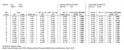
Many are not aware of the major differences between the orifice sizes and discharge coefficients suggested by the API and the actual, ASME values used by the relief valve vendors. According to API-520, Part 1, the API orifice sizes and discharge coefficients are assumed values and are to be used only for the initial selection of the relief valve. They were developed to facilitate choosing a relief valve size early in a project and to ensure that the relief valve finally purchased will have a certified capacity that meets or exceeds the required relief capacity.

However, the differences in capacity between the initial choice of API orifice and the actual ASME orifice can be significant. For most projects, the actual ASME orifice can provide a much greater flowrate. When one also considers the following:

  • Conservatisms in estimating the required relief loads;
  • Calculated orifice sizes are usually between the standard, letter designated API sizes. When this occurs, the next larger orifice size is chosen resulting in the valve being oversized with just an API orifice;
  • The certified ASME discharge coefficient is derated by a factor of 0.9 resulting in another potential source of over design;

the final, purchased, relief valve can be greatly oversized.

The attached table, compares just the differences between orifice designs for two relief valves versus an initial, API design. The first column is the API letter designation for the orifice, followed by the API and then the ASME orifice areas in the next two columns. The fourth column shows that, just based on orifice size, except for the “T” orifice, the ASME orifice flow area is about 16% higher than the API area.

One also needs to consider differences in valve discharge coefficients. Columns 5 and 6 show the (A * Kd) API values. Note that one should not mix and match the orifice areas and discharge coefficients. The API Kd should only be used with the API area – the same with ASME values.

Two actual relief valves are compared in the table. One is a Dresser liquid relief design with orifice areas the same as the ASME designated ones. Since many vendors have valves with areas different than ASME, the second valve is a Farris liquid relief design with orifice sizes as shown. The certified discharge coefficients are also shown for both valves.

The table shows the Farris valve to have a flowrate about 20% higher than the API valve for all sizes except “T”.  It also shows the flowrate from the Farris valve can be higher by as much as 64% for a “D” orifice. The columns next to the flow ratio for both valves show estimated pressure drop ratios which were taken just as the flow ratios squared.

PROCESS ENGINEERS BEWARE!

As shown, the actual pressure drops for the Dresser valve, using actual flow capacity can be higher than those estimated with the API flow capacity by about 44%. But, with the Farris valve, the pressure drop could be higher by a factor of 2.7!  And this does not account for conservatisms in estimating the relief load, extrapolation to larger orifice sizes, or derating of the discharge coefficient.

If not recognized early in a project, both the inlet and outlet relief valve piping could be significantly undersized as well as any downstream relief valve outlet disposal facilities (flare, scrubber, catch tank, etc.).  Issues with acoustically induced and flow induced vibration of the piping may be missed. Emissions from the disposal facilities could also be underestimated, potentially undermining any early permitting activities. All of these could result in a significantly higher capital cost for the project if not captured early.

Consideration should be made to using the ASME orifice sizes during front end engineering.

MINIMIZING PROCESS RISKS / MAXIMIZING CONFIDENCE IN YOUR CAPITAL INVESTMENTS

Overview

When executing capital projects, small or large, the ultimate objective is to produce something that works as planned, at the lowest possible cost, with the most commercially desirable attributes, and meet all applicable laws and standards.  In other words, maximize the return on investment while minimizing health and safety concerns.  To do this, it is extremely important that process risks are identified and managed in the early phases of a project to ensure that the design is robust and that project goals can be met.

Process Risks – Definition/Impact

What is a “process design risk”?  This is a risk associated with the process design that would result in the potential for a new or modified process to fail to meet the overall project objectives.   Whether the objective is to produce a new material scale up an existing process, optimize an existing process to create a better product, or simply produce a saleable product from an existing byproduct or waste stream, the decision to invest in the project assumes that a specified amount of capital investment will result in an expected amount of monetary return.   Process risks, if not identified and managed early in the project, can easily jeopardize its success and result in significant disappointment for the project owner, investors, and even product clients.

Some specific examples of process risk areas:

  • An accurate, detailed accounting of all mass and energy associated with the process has not been completed – raw materials, intermediate products, utilities, internal recycle loops, effluent waste streams, and emissions.
  • The data used as the basis for the design calculations are not robust enough to support the design (e.g. actual vapor-liquid equilibrium (VLE) data is not available, the data used for scale-up of the process did not include the correct correlations, or there was insufficient lab/pilot run-time to support the consistency of the data).
  • Sensitivity analyses are needed to define key variables that could significantly impact the detailed design of a key piece of process equipment (e.g. reflux ratio versus number of trays)
  • The unit operations required to make the product would involve multiple steps and for one or more these steps the equipment is not yet well-defined or not yet proven on a commercial scale.
  • The availability of raw materials in the quantity/quality required has not been confirmed.

These and other process design issues need to be identified and managed early in the design lifecycle of a project.  Failure to do so could result in one or more the following impacts:

  • Inability to produce a product of specified quality or at a specified throughput.
  • Generation of greater than expected effluents for discharge or treatment resulting in excessive treatment/disposal costs
  • Generation of greater than expected emissions resulting in failure to meet applicable permit limits
  • Use of more raw materials than expected resulting in higher than expected operating costs
  • A greater than expected utility requirement that not only results in higher than expected operating costs, but also requires additional capital expenditure because the existing utility infrastructure is inadequate.

All of these will result in a hit to the bottom line, not to mention wasted time, wasted resources, lost revenue, and damaged reputations.

 How to Manage and Minimize the Risks

Minimizing process design risks involves a systematic, rigorous examination of the quality of the process design.   The engineer needs to know what questions to ask, what to look for, and be able to identify all the ways that the process could potentially fail to meet the process objectives.

 Preliminary Process Design PhaseIn the early stages of a project, it is critical to perform a detailed process analysis to validate the technical feasibility of the proposed system and accurately define the major equipment and system configuration(s) that would meet the desired objectives. The information developed at this phase will provide specific insight on whether it can be done, what challenges need to be addressed for it to be successful, and how much it will really cost.

Most critical is the development of a sound Process Design Basis document as well as a detailed Heat and Material Balance (HMB) for the system.  The Process Design Basis document summarizes the raw material and product specifications, plant capacity requirements, available utilities, critical plant operating parameters that would impact the design, specific unit operations performance requirements, applicable regulatory requirements, and any other goals and/or constraints desired by the owner/operators/engineers.  Once this is in place and agreed upon by the project team, the process engineers can go to work to create, analyze, and optimize, to the extent possible, the process design.  The HMB is generated to determine the feasibility and evaluate various configurations.  It is recommended that appropriate process simulation software tools be used for this task.  The speed and accuracy of process simulation can save tremendous time and money during the preliminary design phases by allowing more efficient evaluations of various cases; e.g. plot of reflux rate versus energy usage or versus number of trays; plot of recycle rate versus yield, etc.

The design basis and HMB information allows the experienced process engineer to specifically define additional data needs, sensitivity analyses, technical and economic process alternative evaluations, and vendor or pilot testing needed to confidently design an optimized system.     These are tasks that should be executed prior to (or sometimes in parallel with) the development of detailed process design documents.  A precise manageable explanation of the work to be done in these tasks should be documented.

It is widely recognized that this key front-end work will have a major impact on the overall project and ultimate operation of the process. If this work is not done properly, then the project is in trouble no matter how well the subsequent detailed engineering, construction, and project management work are executed.  This information, along with a financial analysis, can be used as a sound basis for making decisions – does it makes sense to proceed? If so, what key issues need to be considered along the way?

Detailed Process Design PhaseAt this point the major process design risks have been identified and preliminary design documents have been generated – now the system components need to be integrated together to ensure the design intent can be met.  This will include such things as incorporating critical process details into the equipment specifications, developing piping and instrumentation diagrams (P&IDs) and a control scheme with consideration of all operating scenarios (startup, normal operations, shutdown, emergency shutdown).  The experienced process engineer continues to evaluate the process for how it could potentially fail and develops the best practical solutions.  After review and selection of a solution by the team, the engineer makes sure that the process design documents accurately capture these important details.

Some examples of process risks that can be mitigated during this phase include:

  • A detailed evaluation of the vent header hydraulics shows the need for a booster fan in the existing vent line to accommodate the additional load or rerouting of the vent header to another area.
  • An evaluation of the startup scenario for a specialty reactor identifies the need for an additional small heating source until the process comes to temperature or configuring the process for use of recovered heat somewhere else in the facility.
  • A review of potential upset conditions results in the need for either a small polishing filter or additional measurement devices so that permit requirements can be continuously met.

These are just a few examples of critical items that might be captured during the detailed process design phase.

Detail Engineering/Procurement/Construction Phases – Sometime during, or at the completion of the detailed process design phase, the detailed mechanical, electrical, and civil/structural design begins (detail engineering).  A well-developed detailed process design package is a critical component to the success of the detail engineering design.    Although the process engineer’ role in this phase is significantly reduced, it is critical to include them as the design progresses so that the integrity of the process design is preserved.   As companies try to keep a competitive advantage, there is great pressure to hold down costs as the civil, mechanical, electrical and instrumentation details are developed.   Removing a component that may seem unimportant can lead to the potential for off-spec product, reduced throughput, or higher operating costs.  The process risks are managed in this phase by ensuring that the experienced process engineer is present in the project reviewing drawings, equipment selection, developing operating procedures, etc.

Summary

Managing process risks through the design lifecycle of a project will greatly enhance the probability that the new or modified system will operate with the intended outcome.   The process engineer (or engineers) should have the applied design knowledge and the experience to both know how to identify the risks and design to minimize or eliminate them.  This allows the project owner can to confidently make decisions every step of the way.

2018 PHA Training Course Offered by PROCESS

PROCESS ENGINEERING ASSOCIATES, LLC is pleased to publicly offer the following 3½-day PHA training:

PROCESS HAZARD ANALYSIS (PHA) LEADER TRAINING COURSE

The purpose of the 3½ -day training course is to assist personnel at chemical plants, petrochemical plants, petroleum refineries, and manufacturing plants in becoming proficient in leading and documenting process hazard analyses (PHAs) by becoming familiar with various qualitative hazard review techniques and industry best practices for conducting and documenting PHAs.

Who should attend:  Managers and engineers responsible for conducting PHAs at chemical plants, petrochemical plants, petroleum refineries, and manufacturing plants.

Detailed instruction of the following hazard review methodologies will be included in the course:

  • Hazard and Operability (HAZOP)
  • What-If
  • Checklists
  • Failure Modes Effects Analysis (FMEA)

An introduction to Layer of Protection Analysis (LOPA) will also be included.

Select from the following course locations:

  • Houston, Texas
  • Portland, Oregon
  • Tulsa, Oklahoma
  • Philadelphia, Pennsylvania
  • Denver, Colorado
  • New Orleans, Louisiana

Please visit our website here for detailed course information and registration.  We hope to see you there!